On The Road To St. Petersburg

Let me tell you a story.

When I was a young man, I lived for a time as an itinerant gambler, wandering the Russian countryside to engage my fellows in games of chance. Although I was known to gamble on cards, dice, and animals, my favorite game was played with nothing more than a simple coin. The rules of my game were as follows:

You may place a wager of any whole number, e.g. 5₽. I will flip a perfectly-fair coin, and if it comes up heads, I will pay you the value of the wager, plus an extra 20%. If the coin comes up tails, I will keep the money you wagered. Afterwards, you have the option to place a new wager and play again. You may continue to play until the sun rises above the horizon.

In the summer of my twenty-third year I journeyed on the road from Moscow to St. Petersburg, peddling my games along the way. One fine afternoon, I set up my booth in the city of Expectsibirsk, a legendary metropolis populated entirely by perfectly rational expected-value maximizers. A man named Evan wandered over with 100₽ in his pocket. Upon reading the rules, Evan performed the following calculation.

“For every ruble wagered, there is a 50% chance of winning 1.20₽, and a 50% chance of losing 1₽. In expectation, this will net 0.10₽ per ruble wagered. The expected value improves with each ruble, so the more rubles wagered, the better. I wager all 100₽.”

I flipped my coin and…heads! Now, Evan had 220₽. Reading once more the rules of the game, he said,

“Well, once again, for every ruble wagered, I expect to win 0.10₽. This situation is just the same as it was a moment ago, except I have more money available to gamble with. I bet 220₽.”

Heads again!

“I bet 484₽.”

Another heads!

“1064₽.”

…and, at last, a tails. Evan walked away with 0₽ in his pocket, but with his head held high.

“I just made a fortune in expected rubles.”

Evelyn greeted me next. She made 1,000₽, then lost it all…including the 500₽ she started with. Everett was less lucky; his first flip was a tails, and I grew 10,000₽ wealthier. But saddest of all was poor Everly, who began her game with a handful of coins, amassed a fortune of billions of rubles, and then lost it all in an instant.

Nobody ever walked away from my game, or wagered even a single coin less than the sum total of their personal wealth. After all, the dictums of EV maximization held that to do so would be irrational. And so, with each participant, I flipped my coin until they lost, and pocketed their initial wager. As night fell, I carefully packed away my earnings and slipped out of town, before the mobs of newly destitute could locate the source of their woes.

But as I departed Expectsibirsk, I encountered a boy dressed in rags. By my garb, he recognized me as a gambling man, and requested that I allow him to tempt his fortune. Although my pockets were already full, for love of the game, I acquiesced. After reading my rules, the boy spoke.

“I will wager 10₽.”

I dutifully flipped my coin, observed the heads, and paid him his rightfully-earned 12₽.

“I will play again. 10₽.”

Had I misheard? No – the boy extended his hand, a ten-ruble coin resting in his palm. Very well, I thought to myself, flipping my coin. This time, the coin turned tails, and I pocketed his 10₽.

“Once more, again for 10₽.”

Lady luck smiled upon me, and the boy parted with his 10₽. As I pocketed the coin, I turned to go.

“10₽.”

I glanced up sharply. He had lost his initial bankroll, yet continued to play? Had the boy been holding money in reserve? Squinting at his gaunt physique, I realized that what I had taken for an unsightly tumor on his leftward side was in reality a satchel strapped beneath his rags, filled to the brim with ten-ruble coins. For the first time since arriving in Expect, I spoke.

“What is your name, boy?”

“Tenjamin.”

For the rest of the night we gambled. Sometimes he won, sometimes he lost, always the boy wagered but a single 10₽ coin. By the time the sun rose to free me from the game, he had taken everything I won in the city, and much more besides. To this day, I am still paying off the debt I accrued on the road to St. Petersburg.

The St. Petersburg Paradox

Should one always choose the action with the highest expected value?

Many people believe so. It’s a beautiful idea: incredibly powerful, and yet elegant in its simplicity. For intellectually-minded folk, there’s something wonderfully compelling about a guideline that can be applied universally. Any decision-making scenario becomes reducible to a mathematical exercise. Simply map each outcome to a scalar measure of value, estimate the probabilities, marginalize, and ride forth — confident that you have chosen the best option that your current knowledge allows.

As a rational-minded person myself, I see the appeal of this perspective. But expected value has an ugly side, too. Sometimes, expected-value maximization can lead to strange, unintuitive decisions, and as we saw in my story, following its dictums can lead to ruin. What’s going wrong? Is there a way to fix it?

Many situations where expected value have trouble share a common source. The St. Petersburg paradox is a well-known statistical conundrum, one which beautifully distills the heart of the issue. The paradox concerns a particular gamble, which I’ll call the doubling game.

Here are the rules. The game begins with $2 in the pot. The player repeatedly flips a fair coin. Each time it lands heads, the amount of money in the pot doubles. The first time it lands tails, the player is given the money in the pot, and the game ends.

What is the most that a rational gambler should be willing to pay to play this game? Clearly, the answer is at least $2, because that’s the minimum payout. But we will sometimes see a long sequence of heads, and the payout will be much higher, so perhaps we should be willing to pay more.

Expected-value maximization gives a clean numerical answer to this question. According to the EV framework, the amount that a gambler should be willing to pay is equal to the expected value of the game’s payout. We can compute this easily, by partitioning the outcomes based on the number of flips. There is a \(\frac{1}{2}\) chance of seeing exactly one flip (if the first flip is tails), a \(\frac{1}{4}\) chance of seeing exactly two flips (heads, then tails), a \(\frac{1}{8}\) chance of seeing exactly three flips…the pattern is clear, the chance of seeing \(n\) flips is \(\frac{1}{2^{n}}\). And what are the values of these outcomes? \(2,4,8,16,...\)so \(n\) flips nets \(2^{n}\) dollars. Marginalizing, we see that the expected value is \(\sum_{n=1}^{\infty} 2^{n}\left(\frac{1}{2^{n}}\right) = \sum_{n=1}^{\infty} 1 = \infty\). Hmm.

Now, “infinity” is not really a number, so one must generally be a bit careful reasoning about results which include infinities. In this instance, the conclusion can be straightforwardly understood as “the expectation is larger than any finite number”. So the answer to our question is: a rational gambler will be willing to pay any finite amount of dollars to play this game.

Of course, paying \$1,000,000,000 to pay this game seems like quite a stupid thing to do. Hence: paradox.

Many people have proposed resolutions to this paradox, most prominently utility theory¹ and default risk.² But I find these to be very unsatisfying. They merely assume away the existence of situations that would be problematic, without addressing the fundamental issue.

To be honest, I don’t think “paradox” is even quite the right description here. There’s no fundamental inconsistency at play. This is just an example of a situation where the expected-value framework is ineffective. Choosing to play the doubling game with a buy-in of \$1,000,000,000 really does have positive expected value, and really does lose you money. There’s nothing paradoxical about the fact that a decision-making framework can be bad, sometimes. Many people treat expected-value maximization with something akin to reverence, elevating it as the pinnacle of rational behavior; but at the end of the day, it’s just a decision-making rule. And is it a paradox when a decision-making rule like “go with your gut” leads to losing money in some situations? Of course not – “go with your gut” is just a bad rule. And it turns out that expected value is similarly flawed, although its issues are far more rare and subtle.

A real resolution to the St. Petersburg paradox requires an improved decision-making framework.

Maximize The Realizable Value

Here is my proposal: take the action that maximizes the realizable value.

The realizable value³ of a bet, or RV, is the amount of money that you will end up winning if you play enough times. In other words, it is an outcome whose probability gets more and more likely, the more times you play the bet. It is defined using a well-understood concept from probability theory known as convergence in probability. If the ratio between the outcome of repeatedly taking a bet \(X\), and some expression \(z\), converges in probability to 1, then that bet is said to have a “realizable value of \(z\)”, and denoted \(\mathbb{R}[X_{1..n}] = z\).

By deciding whether or not to take a bet based on its realizable value, we are essentially reasoning about what would happen if we played the bet repeatedly. However, it’s still perfectly coherent to apply this decision rule to bets that are just encountered once. The philosophy endorsed by an RV maximizer is “I should play this bet now if I would be happy to play it forever.”

One important subtlety to note is that while expected value is a property of an individual wager, convergence in probability is actually a property of a sequence of wagers. When we refer to the realizable value of a wager \(X\), keep in mind that this is merely shorthand for the realizable value of a sequence of \(X_{1..n}\) where each \(X_i\) is an identical copy of \(X\). In general, it’s not the case that all the \(X_i\) need to be the same.

If you’ve never studied probability theory, you might be a bit confused by how this definition of realizable value is different from the familiar notion of expected value. Maybe it feels like just an unnecessarily-complicated way of expressing the same concept. This is a reasonable first impression, because the difference between the two frameworks is subtle. In fact, for all bets with finite expected value, the weak law of large numbers tells us that these two concepts are exactly the same: the long-run average payout of a repeated bet will converge in probability to its expected value. This means that the realizable value of any bet with finite expected value is basically just its expected value! Thus, all of your intuitions from expected-value maximization carry over to realizable-value maximization.

But when a bet has infinite expected value, the two frameworks sometimes come to different conclusions about what actions to take. This true for the St. Petersburg paradox, and also plays an important role in my story about Expectsibirsk. In a moment, we’ll walk through these examples in more detail.

Personally, I find it to be quite cool that RV matches up perfectly with EV in all the situations we know that EV feels correct, and gives a new answer in precisely those situations where EV does something weird. But it’s not as though I carved out specific exceptions: this approach is unified and natural, but just happens to do exactly what we would want. Isn’t that elegant?

Before we go on, let’s build a bit of intuition as far as what it might look like when the expected value and realized value are not the same. On the surface, it seems a bit surprising that this is possible. How can the two be different? How can we on average make an infinite amount of money, but still be guaranteed to make a finite amount of money?

The archetypal setup for this weirdness is when some extremely-unlikely outcomes have massive value. For example, consider playing many rounds of a 50/50 2.2x-all-or-nothing bet, like the one I offered in Expectsibirsk, starting with \$1. After 100 rounds, the chance that you have exactly 0 dollars is \(1-(.5)^{100} \approx 1-10^{-30}\). But! If you do find yourself with some money, then you will have made \(2.2^{100} \approx 10^{34}\) dollars. Since, in each round, the amount of money that you could make is growing faster than the likelihood of that outcome is decreasing, the expected value of this strategy grows infinitely as more rounds are played. But the chance that you walk away with nothing is also growing to approach 100%, and in the end, that’s always what happens.

So if you are acting to maximize expected value, like the citizens of Expectsibirsk in my story, you would play this game. But if you were acting to maximize realizable value, you would not.

Next, let’s walk through some examples of realizable value in action. In each scenario, we are invited to play a particular game for \(n\) rounds, and ask: what is the fair price? In each example, \(X_i\) denotes the random variable that refers to the outcome of the \(i\)th round, so our average payout for \(n\) plays is \(\frac{1}{n} \sum_{i=1}^{n} X_i\).

Basic coin flip.

The player flips a fair coin which pays out \$10 for heads and \$0 for tails.

The expected value of any round \(\mathbb{E}[X_i] = 0.5(10) + 0.5(0) = 5\) for all \(i\). Since this is finite, the weak law of large numbers tells us that \(\left| \mathbb{E}[X_i] - \sum_{i=1}^{n} \frac{X_i}{n} \right| \overset{P}{\to} 0\) as \(n \to \infty\), or equivalently, \(\sum_{i=1}^{n} \frac{X_i}{n\mathbb{E}[X_i]} \overset{P}{\to} 1\). So \(\mathbb{R}[X_{1..n}] = 5n\).

As a realizable-value maximizer, I should be willing to pay up to $5 per round of play. Of course, this coincides with the solution given by expected value.

Doubling game.

The player flips a fair coin until it comes up tails. If the first flip is a tails, the payout is $2, and for each heads seen, the payout doubles.

As we saw above, \(\mathbb{E}[X_i] = \sum_{n=1}^{\infty} 2^{n}\left(\frac{1}{2^{n}}\right) = \sum_{n=1}^{\infty} 1 = \infty\). But as it turns out, \(\mathbb{R}[X_{1..n}] = n \log_2 n\). The math here is a bit more involved, so I’ll just give the high-level intuition of the analysis. If you are comfortable with probability theory, a rigorous proof is given by Dunnet in his textbook (Example 2.2.16), or more explicitly in Sebastien Roch’s lecture notes.

The key tool is our ability to truncate a random variable, meaning clip its value to 0 if it falls outside of a certain range. Truncation is helpful for this sort of problem because, once we have truncated, the expectation is guaranteed to be nice and bounded. Denote the truncation of a random variable \(X\) to the level \(b\) as \(T(X, b) = X \cdot \mathbb{1}_{|X|<b}\) (where \(\mathbb{1}\) denotes the indicator function that is equal to 1 if its condition is true, otherwise 0).

What’s cool about truncation is that truncating a random variable does nothing if the value of that variable turns out to be less than the truncation threshold. By gradually increasing the truncation threshold, we can make it less and less likely that truncations have any effect at all. Therefore, we can understand our sequence of \(X_i\)s as the limit of a sequence of sequence-of-truncated-\(X_i\)s, where the truncation levels get less and less strict. As the truncation threshold grows, we end up with almost no probability that any variable actually gets impacted.

Concretely, define a sequence of truncation levels \(t_j = j \log_2 j\). For each level \(t_j\), we truncate the first $j$ terms of our sequence of \(X_i\). A bit of algebra leads to the conclusion that \(\sum_{i=1}^j \mathbb{P}(X_i \neq T(X_i, t_j)) \to 0\) as \(j \to \infty\), meaning that we eventually see that there is almost no chance that any variable will get truncated.

Next, we just need to analyze the truncated sequence. We know that the expectation and variance for truncated variables exist, and for any particular sum of \(j\) variables truncated at level \(t_j\), some more algebra tells us that the expectation \(\mathbb{E}[\sum_{i=1}^j T(X_i, t_j)] = j (\log_2 j + \log_2 \log_2 j)\), which we can denote as \(\mu_j\). After checking some conditions, we can use Chebyshev’s inequality to bound the probability that the actual sum deviates from this mean by a factor of more than \(t_j\), leading to the conclusion that \(\frac{|\mu_j - \sum_{i=1}^j T(X_i, t_j)|}{t_j} \overset{P}\to 0\) as \(j \to \infty\).

Since both (1) the truncated sequences converge in probability to the real sequence, and (2) the deviations of the sum of the real sequence converge in probability to 0, we can conclude that the deviations of the sum of the real sequence converge in probability to 0. Thus, for a real sequence of length \(n\), we have \(\frac{|\mu_n - \sum_{i=1}^n X_i|}{t_n} \overset{P}\to 0\) as \(n \to \infty\). Plugging in \(\mu_n = n (\log_2 n + \log_2 \log_2 n)\) and \(t_n = n \log_2 n\) and doing a bit more algebra gives \(\sum_{i=1}^n \frac{X_i}{n \log_2 n} \overset{P}\to 1\), and thus, \(\mathbb{R}[X_{1..n}] = n \log_2 n\).

Whew. Let’s marinate for a moment on the implications of this result. It seems that in the doubling game, the realizable value per round grows with the number of rounds being played. If you’re only playing 1000 rounds of the game, the amount that you are willing to spend is \(1000 \log_2 1000\), so you value each round at \(\log_2 1000 \approx\)\$10. But if you are playing 100,000 rounds, then suddenly you value each round at \(\log_2 1000000 \approx\)\$20! It’s as though this game has an inherent economy of scale. The more times you play, the more valuable each play becomes.

To me, this is a completely satisfying resolution to the St. Petersburg paradox. We didn’t alter the situation at all, just directly tackled the problem as it was initially presented. We used a generic, first-principles approach, not anything problem-specific, and with no free parameters. We ended up with a concrete answer, assigning a specific numerical value. And the answer elegantly synthesizes our two intuitions – that on one hand, the game has the potential to be extremely valuable, but on the other hand, a single play is not worth much.

To double-check this result, I ran a simulation (code) of two billion doubling games, computing the mean reward per game over time:

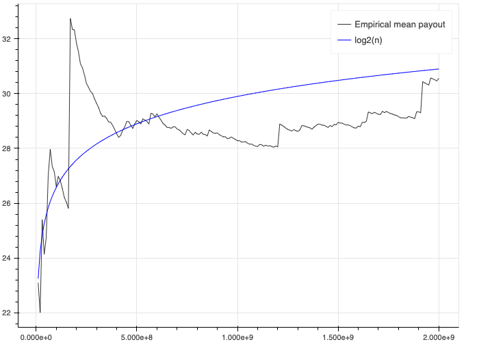
A bit noisy, but overall pretty convincing.

Wagering game.

The player has a bankroll of \(b\) dollars, and wagers \(fb\) dollars where \(0 \leq f \leq 1\). The player flips a coin, which comes up heads with probability \(p\). If heads, the wager is multiplied by some factor \(1+w\) for \(w > 0\). If tails, the wager is reduced by some factor \(1 - l\), where \(0 < l \leq 1\).

The expected value of each round of this game is \(pfbw - (1-p)fbl = fb(pw - (1-p)l)\). So, as long as \(pw > (1-p)l\), each round has an expected value which is linear in the bet size, and so the expected value is maximized by betting everything. (Otherwise, the bet is expected to lose money, and value is maximized by betting nothing.) In fact, thanks to linearity of expectation, it’s possible to prove that this also holds true for sequential bets: when \(pw > (1-p)l\), or equivalently, \(\frac{pw}{(1-p)l} > 1\), we maximize the expected value after \(n\) rounds by betting everything, every time.

What value is realized by this strategy of always betting everything? Let \(H_n\) be the number of heads seen after \(n\) rounds, and so \(n - H_n\) gives the number of tails. This means that the bankroll \(b_n = b_0(1+w)^{H_n}(1-l)^{n-H_n}\) at timestep \(n\), where \(b_0\) gives the initial bankroll. Since \(\mathbb{E}[\frac{H_n}{n}] = p\), the law of large numbers tells us that \(|\frac{H_n}{n} - p| \overset{P}\to 0\) as \(n \to \infty\). We can use this fact to show convergence in probability of the average log-wealth. For the bankroll \(b_n\),

as \(n \to \infty\). From here, we can use an epsilon-delta argument to verify that \(\frac{\log b_n}{n} \overset{P}\to z\) implies that \(b_n \overset{P}\to 0\) if \(z < 0\), so its realized value is $\(-b_0\). And so we see that this strategy will realize gains if and only if \((1+w)^{p}(1-l)^{(1-p)} > 1\).

In summary, EV says to bet it all if \(\frac{pw}{(1-p)l} > 1\), whereas RV says to bet it all only if \((1+w)^{p}(1-l)^{(1-p)} > 1\). Unfortunately, these two conditions do not always agree. For example, when \(p = .5, w = .6, l = .5\), we see \(\frac{pw}{(1-p)l} = \frac{.5(.6)}{.5(.5)} = 1.2 > 1\), while \((1+w)^{p}(1-l)^{(1-p)} = (1.6)^{.5}(.5)^{.5} \approx .89 < 1\).

This result explains trouble for the citizens of St. Petersburg in the story at the beginning of this essay, who were offered a bet with \(p = .5, w = 1.2, l = 1\). Plugging into the EV condition gives \(\frac{pw}{(1-p)l} = \frac{.5(1.2)}{.5(1)} = 1.2 > 1\), so they chose to bet all of their money, but \((1+w)^{p}(1-l)^{(1-p)} = (1+1.2)^{.5}(1-1)^{.5} = 0\), so their realized outcome was \$0. They would not have lost their money had they had aimed to maximize their realizable value instead of their expected value.

Of course, these conditions are not about the value of the game itself, only about the value of the bet-it-all strategy. By betting differently, it is still sometimes possible to win. For example, Tenjamin wagered in such a way as to play the “basic coin flip” game, so he was able to realize earnings of \(1.2n\): his realized wealth grew linearly as long as the game continued. That’s already a big improvement over earnings of -$\(b_0\). But could he have done even better?

In fact, our analysis reveals a straightforward way to identify an optimal betting strategy. If the bet in each round were \(z_n = f b_n\) for some fraction \(0 \leq f \leq 1\), such that the payoff for winning decreases to \(fw\) and the penalty for losing decreases to \(fl\), we see \(\frac{\log b_n}{n} \overset{P}\to p \log (1+fw) + (1 - p) \log(1-fl)\) as \(n \to \infty\). To identify the strategy with the fastest growth rate, all we need to do is choose the \(f\) which maximizes this value, which can be done by setting its derivative equal to zero and solving the resulting equation. The solution, \(f^* = \frac{p}{l} - \frac{1-p}{w}\), is the formula for the famous Kelly Criterion.

One last interesting property to note: EV and RV agree when \(f\) is very small. This means that we only need to take RV into account when wagering a non-insignificant fraction of our bankroll. For tiny bets, reasoning with EV is sufficient. To see this, we need to use the fact that \(\log x+1 \approx x\) for \(x \approx 0\). Recall that EV says that we should take the bet when \(\frac{pw}{(1-p)l} > 1\), and RV says that we should take the bet when \((1+fw)^{p}(1-fl)^{(1-p)} > 1\).

Starting with the condition for when the wagering game has positive RV:

we can take the log of both sides:

Now, using the fact that \(f \approx 0\), we have \(fw \approx 0\) and \(-fl \approx 0\), so:

\(\log \left( (1+fw)^{p}(1-fl)^{(1-p)} \right) = p\log(1+fw) + (1-p)\log(1-fl) \approx p(fw) - (1-p)(fl)\).

Substitute this approximation into our inequality:

and then rearrange:

and we’ve shown that the condition for when a bet has positive RV is identical to the condition for when a bet has positive EV, when \(f\) is sufficiently small.

Connections

Another sign of a good framework is if it explains the world well. One would expect a good decision-making rule to pop up in all sorts of places, being used implicitly, even before being formally understood. I want to highlight a few places where I’ve noticed that reality coincides with the dictums of realizable-value maximization.

Gambling

We’ve just discussed how the Kelly Criterion can be derived through the lens of maximizing realizable value. Interestingly, as far as I can tell, the original motivation was nothing of the sort. The Kelly Criterion was initially derived for an ad-hoc objective: maximizing the expected logarithm of wealth. Later, it was shown to also be equivalent to maximizing the geometric rate of return.

These are perfectly valid goals, but they fall short as complete decision-making frameworks, since they don’t provide any characterization of when they should be invoked (why maximize expected wealth sometimes, and expected log-wealth other times?) and are limited in their scope (the Kelly criterion does not explain how much to pay to play the doubling game).

I’ve always found the Kelly Criterion to be a beautiful strategy, but I was never quite at ease with its ad-hoc-ness. I think it’s amazing that the framework of realizable-value maximization serves to motivate it from first principles. Also, the Kelly Criterion is a widely-used approach, vouched for by professional investors and gamblers alike; the fact that it coincides with the optimal realized value is a strong point in favor of the practical usefulness of this framework.

Psychology

It’s conventional wisdom in economics that humans have logarithmic utility functions. This is, for example, the motivation given by Kelly to maximize log-wealth in the first place. Empirical experiments seem to mostly corroborate this, although it is possible a different functional form may be a somewhat better fit. Economists simply accept logarithmic utility as a premise, and build from there.

With realizable-value maximization in mind, this perspective reverses. We can now answer the question: why do humans have logarithmic utility at all? Here’s my thinking.

It’s a reasonable assumption that wealth is generally helpful for survival, especially when we broaden the definition of wealth beyond just fiat currency: power, status, prestige, possessions, etc. This implies that evolutionary pressures should have instilled in us good instincts for accumulating wealth over the course of our lives. Obviously, genetics are not fine-grained enough to instill theoretical knowledge of realizable-value maximization. But what it can do is give us instincts that, when followed, allow us to implement a RV-maximization algorithm. Which, perhaps, explains why humans have logarithmic utility.

It may be a coarse model, but overall, I think it’s pretty reasonable to view life as a big, long-horizon repeated betting game, always played using the same bankroll. We know that logarithmic utility maximization is identical to following a Kelly strategy in the specific setting in which that strategy is applicable, and it is very likely that it has connections to RV-max in general. So by living according to logarithmic utility, we are able to realize the most wealth over our lifetimes, and survive and reproduce.

Conclusion

We’ve seen the problems with expected value, and how realized value naturally resolves them. But does this mean realized value is a better decision-making framework than expected value?

It’s a challenging question, because it’s fundamentally philosophical. Within the context of a specific framework, it’s straightforward to identify which choices are superior. Indeed, that’s the whole purpose of a framework, which is at its core nothing more than a way of inducing a ranking over choices.

But comparing between frameworks is an entirely different ballgame. There’s no external, objective metric that will tell us which is the best. We’re forced to invoke subjective arguments: about which frameworks make the most sense, seem like they work well, or just “feel right”. For people who consider themselves objective, rational decision-makers, this can be an uncomfortable realization.

Personally, I am sold on the idea of maximizing realizable value instead of expected value. I find it elegant, natural, and well-aligned with my intuitions. Hopefully, those of you who are still with me at this point are also on board. And for those that aren’t – I am excited to hear your counter-arguments.

That being said, I would be surprised if realizable-value maximization is the end of the story when it comes to decision-making frameworks. Most likely, it has its own subtle issues, and given enough time, a paradox will rear its ugly head once more. When that happens, I will be right there alongside everyone else striving to replace RV with an even better decision-making framework.

The final question is: how does understanding realizable value impact our decision-making?

The biggest change is that we need to view our decisions more holistically. Expected value considers each bet in isolation, but realizable value considers each bet as just one member of a long sequence. We each have a single bankroll maintained over the course of our lifetime, and in order to maximize its value, we need to place each wager on the basis of how it will affect us, long-term. Similarly, whereas expected value can always be computed for a single play of a game, realizable value forces us to consider that the value is dependent on the amount of times we will be able to play it. It is simply not possible to make good decisions when each individual bet is considered in isolation.

However, in most day-to-day situations, it is unlikely that you need to change much. As we have seen, EV and RV make identical recommendations when the wager is a small fraction of the total bankroll. Small risks can therefore be understood perfectly well through the conventional lens of EV. But major investments or life-changing decisions need to be considered differently. In situations where you will probably be thinking very hard about what to do, realizable value is the proper concept to think about.

Thanks for reading. Follow me on Substack for more writing, or hit me up on Twitter @jacobmbuckman with any feedback or questions!

Many thanks to David Buckman, Carles Gelada, Warfa Jibril, Joel Einbinder, and Tony Pezzullo for their ideas and feedback.