How To Think About Replay Memory

The replay memory, or replay buffer, has been a staple of deep reinforcement learning algorithms since DQN, where it was first introduced. In brief, a replay memory is a data structure which temporarily saves the agent’s observations, allowing our learning procedure to update on them multiple times. Although it is straightforward to implement and understand, the role of replay memory within the overall RL procedure is in many ways non-obvious. Many people, especially newcomers to the field, do not have a strong conceptual understanding of how it impacts learning. This brief blog post will serve to clarify.

Saving vs. Streaming Algorithms

To understand the role of replay memory, I’m going to introduce a new¹ taxonomy of algorithms. We can place any given RL algorithm on a spectrum from saving algorithms to streaming algorithms.

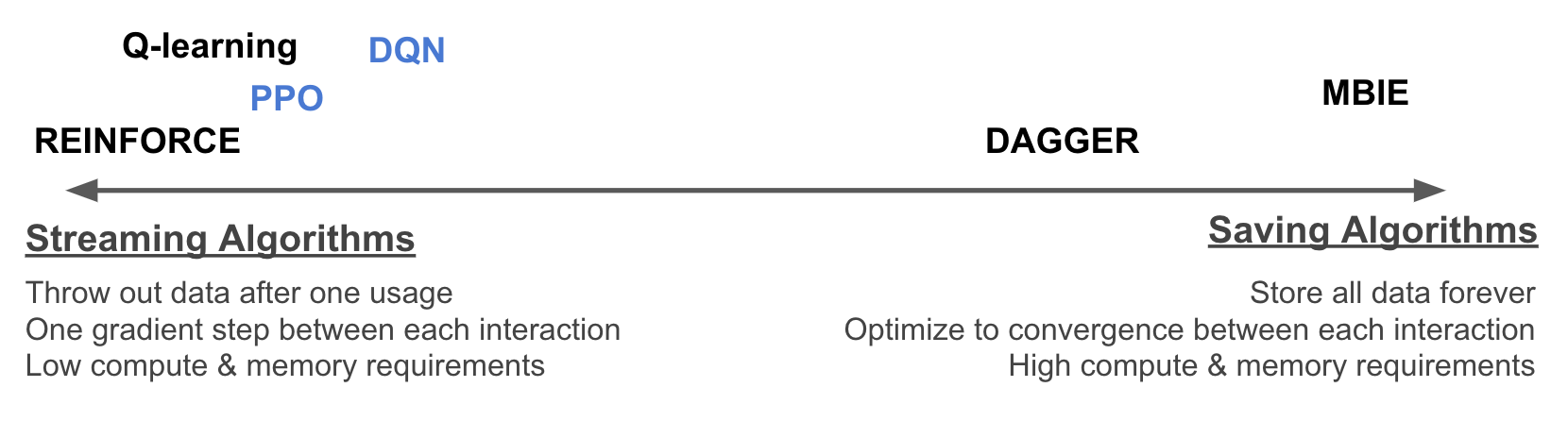
On the streaming end, we have algorithms which acquire an observation, use it to perform a small update to the agent, and then discard it and immediately act again. On the saving end of the spectrum, we have algorithms which “think hard” before acting. Saving algorithms store every single observation, forever. Each time a new transition is observed, the agent is re-trained before it acts again; this means performing arbitrarily many updates, until the agent has fully incorporated the information of all the observations it has ever made. (Also, note that the principles of saving and streaming are to a large degree orthogonal to other taxonomies, such as the policy-based vs. value-function based vs. model-based distinction…all of these frameworks can be used for either streaming or saving algorithms.) One other interesting thing about saving algorithms is that they form a bridge between online and offline RL; a saving algorithm is an online RL algorithm which works by solving a new inner-loop offline RL problem every time it sees a new observation.

With this spectrum in mind, the role of replay memory is clear. Replay memory is a technique for implementing saving algorithms in deep reinforcement leaning settings.² Furthermore, we can interpolate between the two endpoints of the spectrum by adjusting two hyperparameters: the size of the replay buffer, and the number of learning updates per interaction. When these two parameters are small, our algorithm will be nearly streaming; as they each approach infinity, our algorithm will approach saving.

Thus, the impact of replay memory on an algorithm can be seen by understanding the differences between saving and streaming algorithms. (Since understanding the behavior of algorithms at intermediate points along the axis is tricky, we’ll focus our thinking around the two endpoints.) What are the strengths and weaknesses of each of these two types of algorithms? Let’s contrast them across two important dimensions: compute efficiency and data efficiency.

Computational Efficiency. Streaming algorithms have a clear advantage when it comes to compute and memory requirements. A streaming algorithm never stores more than one observation at a time, so it requires very little memory. Also, it performs only one small update per interaction, so the speed of interaction is almost never bottlenecked by the speed of learning. In contrast, saving methods have enormous memory footprints, as the amount of data that needs to be stored grows with each interaction. And since training to convergence may require many updates, saving methods will typically use vastly more compute as well.

Data Efficiency. Saving algorithms have the advantage when it comes to data efficiency (also called sample efficiency). Again, there’s a clear intuitive justification for this: saving algorithms, which store all of their data and train on it a ton, are clearly “squeezing the most information” out of the data they have seen, and are more efficient as a result. One concrete difference we can identify is that the data efficiency of a streaming algorithm is highly dependent on how the learning is set up; for for example, if we choose a learning rate that is very small, streaming algorithms will require many more samples to reach the same performance. In contrast, for saving algorithms, which train to convergence regardless of learning rate, the data efficiency is not impacted. Another thing to note is that in environments where generalization plays a role, saving algorithms allow information in previously-seen transitions to be brought to bear in updating actions at any point in the future. Let’s say on level 1 of a game, the agent observes an enemy enter a code to open a door, but the door itself is unreachable; then on level 19 of the game, the agent encounters a similar-looking door, with a codepad. A saving method could immediately use the remembered information to infer the code correctly. A streaming method would be forced to try random codes until it eventually got it right, which is very data-inefficient. In real-world tasks, I’m pretty sure it’s almost universally the case that we can generalize from past mistakes to future situations, and so we stand to benefit hugely from this effect.

So, each of these has some advantage…which should we prefer in practice? In general, I believe that data efficiency is more important, as I have discussed previously. For one, Moore’s Law has held strong for a while, and even if it is vaguely slowing down, “astronomical compute today is trivial compute tomorrow” is still a good rule-of-thumb. Data collection has no such law. Also, compute can easily be parallellized and distributed, and is (relatively) inexpensive to scale; there’s plenty of good resources for dong so. Whereas data collection in real-world problems is very ad-hoc and problem dependent, often can be done no faster than the speed of reality, and is generally difficult and expensive to scale up. Our bottleneck is almost always going to be data collection, and so data efficiency is of greater importance. Thus, I believe that saving algorithms are likely to be more important for getting RL to work on real problems.

If saving methods are so much more data-efficient, why do the techniques we use in practice look so much more like streaming algorithms? For example, the default hyperparameters on DQN update on each datapoint only an average of only eight times before discarding it. Streaming algorithms have one final key advantage, one which is more subtle: all learning is done using an unbiased estimate of the true environment.

Streaming data come from “fresh” samples every time, so it is impossible to mistake a good action for a bad action, or vice versa (in expectation). But saving algorithms, which reuse a single sample for learning many times, might get completely thrown off. Consider if an action is bad but high-variance, and we’ve only seen it once, but it got “lucky” and happened to appear to be very good. Our agent will think it is genuinely good, and repeatedly update using that information, eventually converging to a policy which performs very badly in the real environment. We can, in theory, fix this by using uncertainty estimates, but nobody knows how to compute uncertainty estimates for neural networks. I wrote an ICLR paper on this issue, which is also summarized in my last blog post.

A Red Herring: On- vs Off-Policy Learning

Before wrapping up this post, I want to talk about how not to think about replay memory. The perspective I’m about to describe is very popular; in fact, it was the motivation originally given by the DQN authors themselves!

To begin, let me summarize the argument made in the original DQN paper, “Playing Atari with Deep Reinforcement Learning” by Mnih et al. DQN is intended to be a deep-learning-augmented version of Q-learning. (Q-learning, by the way, is a streaming algorithm, which performs one gradient update per observation.) In supervised learning with deep neural networks, we typically compute each gradient estimate, not from a single sample, from a large minibatch of samples. The authors wanted to do this for DQN, as well. A natural way to construct a minibatch (say, of size 128) would be to simply interact with the environment for 128 steps, and form a minibatch from all those observations. However, in supervised learning, we want each minibatch to contain IID samples from a fixed distribution; taking 128 samples in a row from an environment would clearly be correlated, and subject to distributional shift. The original motivation for using a replay memory was to “alleviate the problems of correlated data and non-stationary distributions” by “smooth[ing] the training distribution over many past behaviors”.

However, the authors noted, use of a replay memory also introduced some complications. It was here that they made a fundamental misdiagnosis, which has led to so much confusion: they thought that using a replay memory meant that we were doing learning “off-policy”.

To explain why this perspective is wrong, let’s take a closer look at what “off-policy learning” means. A policy is a way to act in the environment. During our learning procedure, we can either collect data according to the policy that the agent currently believes is best – “on-policy” – or we can collect data according to some other policy – “off-policy”. It turns out that collecting data on-policy is crucial to the theoretical convergence of most streaming methods. If our data stream is arriving off-policy, we need to correct for the difference in distributions to make it look on-policy, or else we might fail to ever find anything.

So, why do I claim that it is inappropriate to interpret the complications arising from a replay memory as off-policy issues? After all, the data in the replay memory is sampled from a mix of historical policies, which are different from the current one, right? Why not just fix it with off-policy corrections?

The answer is that the distribution of data when sampling from the replay memory is much worse than just being off-policy. Firstly, the memory distribution has limited support, in the sense that any transitions that do not appear in the replay memory have 0 chance of being sampled, even if they have non-zero probability under some historical policy. This means we can’t correct it to look on-policy. Secondly, when sampling transitions from an off-policy distribution, it is still required that the outcomes (i.e., the resulting reward and next state) are IID conditioned on their inputs (the state and action), from the distribution is given by the dynamics of the environment (i.e., the reward and transition functions). In transitions sampled from the replay memory, this is not the case: if the same transition is sampled out of the buffer twice, its outcomes will also be the same twice, rather than being independent samples from the underlying environment. This distribution does not match the definition of an off-policy data stream.

Fortunately, it does match the definition of a saved dataset, as used in saving algorithms; thus motivating the perspective provided in the first half of this blog post. Off-policy learning is only an issue for streaming algorithms. For saving algorithms, which have different proof techniques and different guarantees, it does not matter whether data is being collected on- or off-policy. (There are some conditions on the data collection; it’s just that on-policy isn’t one of them.) By understanding an algorithm with replay memory as a saving algorithm, we can properly understand its benefits and address its issues.

Conclusion

Hopefully this post convinced you that the saving-streaming spectrum is one of the most useful conceptual tools for understanding reinforcement learning. I personally believe that in order to get practical, sample-efficient, real-world-friendly RL, we will need to move away from the nearly-streaming algorithms we currently use, and towards saving algorithms instead. This will require significant progress in understanding the issues endemic to saving algorithms, which, I believe, is deeply tied to understanding how to properly compute neural network uncertainties.

Thanks for reading. Follow me on Substack for more writing, or hit me up on Twitter @jacobmbuckman with any feedback or questions!