===
Introduction
Hello friends. Today we’re going to be learning about the fundamentals of offline reinforcement learning, which is the problem of choosing how to act based on a fixed amount of data about the environment. This post assumes familiarity with the ideas around standard RL. The goal is to provide interested RL researchers with an overview of the issues that emerge in the offline RL setting, introducing the concepts and results that are most important for understanding and doing research.
The Hard Thing About Offline RL
To begin, let’s take a look at the setting. The name “Offline RL” might make it seem like this setting is best understood as a variant of reinforcement learning. Actually, though, this comparison is a bit misleading: the core issues of RL, such as information gathering and the exploration-exploitation tradeoff, are completely absent in Offline RL. This setting is best understood as a variant of dynamic programming, where the environment is not fully known: “dynamic programming from a dataset”. In regular DP, we are given an MDP $\langle S,A,R,P,\gamma \rangle$, and tasked with finding an optimal policy $\pi^{\ast}$. In Offline RL, we are given only part of an MDP, with the reward and transition functions missing: $\langle S,A,?,?,\gamma \rangle$ We are also given a dataset, $D$.
So, how does this change things? In the dynamic programming setting, there is a well-established formula for computing the optimal policy: the Bellman optimality equation. However, this equation relies on knowledge of $R$ and $P$, which are not available to Offline RL algorithms. The dataset contains transitions observed from the environment, which might give some useful information about $R$ and $P$. However, it also might not – for example, in the case where the dataset is empty, or contains transitions from only a small subset of the overall state space. Thus, it’s clear we need to temper our ambitions in this setting. Rather than attempting to recover the optimal policy $\pi^{\ast}$, our new goal is to find a “data-optimal” policy $\pi_D^{\ast}$, which scores as high as possible, but requires only the information in the dataset. Note that it’s not obvious how best to do this. It’s easy to propose solutions that seem reasonable; for example, we could use the dataset to compute maximum-likelihood estimates of the reward and transition functions, $R_D$ and $P_D$, and then use invoke the Bellman optimality equation on these approximations. But unlike in the dynamic programming case, the resulting policy $\pi_D^{\ast}$ is not guaranteed to be optimal in the true environment. (In fact, as we will later see, this strategy is actually quite bad.)
Thus, the most important questions in the Offline RL setting are very unlike those in the Dynamic Programming setting. In the dynamic programming setting, we know what we are “looking for”. When we compare various DP algorithms, like policy iteration, value iteration, or policy-gradient, we already know that all of these approaches are looking for the same $\pi^{\ast}$. Therefore, we ask questions like, is it guaranteed to find it? what is the convergence rate? what are the computational requirements? In contrast, in Offline RL, we don’t yet know what a good solution looks like. The most important question in Offline RL is: what choice of $\pi_D^{\ast}$ will translate to good performance on the real environment? (Once we have this answered, then we can circle back around and study sample efficiency and whatnot.) So, let’s see what we can say about this.
Let’s start by re-writing the dynamic programming formula for $\pi^{\ast}$ using the Bellman consistency equation, instead of the Bellman optimality equation: $\pi^{\ast} = argmax_\pi Q(\pi)$; $Q^\pi = R + \gamma P^\pi Q^\pi$. In a slight abuse of notation, we’re using $Q(\pi)$ to mean $Q^\pi(s_0)$. Rewriting it this way puts us into a nice framework that can be readily applied to Offline RL, too. We define $\pi_D^{\ast} = argmax_\pi Q_D(\pi)$. Now, the question reduces to: what is the best choice of $Q_D^\pi$? In other words, how should we estimate the value of a policy from data, in a way that leads to us selecting good policies? To understand the answer to this question, let’s take a brief detour and think about a slightly more general one instead.
Detour: Optimization-via-Proxy
Consider an extremely general decision-making problem setting. There is some set of choices $X$; for example, maybe it’s what sport I should play this spring.

There is some objective $J$, which measures a quantity we care about; in this simplified example, it’s a scalar that measures how much fun I will have.
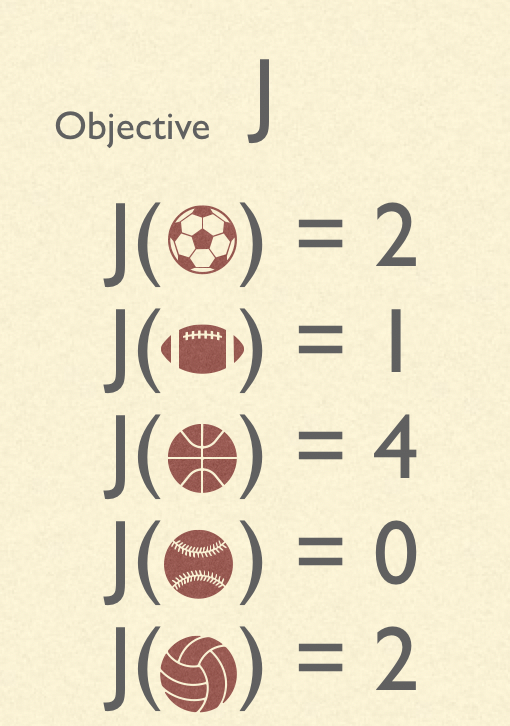
The goal is to choose the $x \in X$ which maximizes $J(x)$. However, the decision-maker doesn’t have access to $J$. After all, I don’t know exactly how much fun I will have doing each sport, and I have to decide what to sign up for now, so I can’t try them out before making the decision. However, the decision maker does have access to some proxy objective $Z$, which will ideally be informative of $J$.
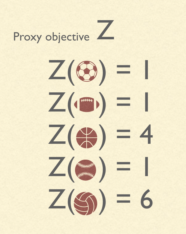
For example, I might survey several of my friends who played sports last spring, and ask them to estimate how much fun they had. Then, I pick the sport with the highest average rating (according to my friends).
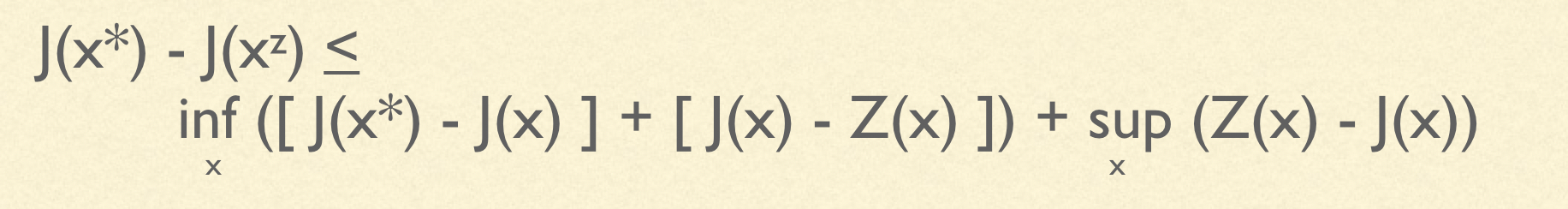
We wish to know: if the decision-maker chooses the $x \in X$ which maximizes $Z$, will my score be high according to $J$? Concretely, if we let $x^{\ast} = argmax_{x \in X} J(x)$ and $x^{z} = argmax_{x \in X} Z(x)$, what will be the regret, $J(x^{\ast}) - J(x^{z})$? Clearly, this regret will be expressed in terms of the similarity between the real objective and the proxy objective. If J and Z are identical, then the regret will be zero. But if they are not identical, then the relationship becomes more interesting:
Let’s take a closer look and see on an intuitive level what this bound is saying. Regret will be small under a specific condition:
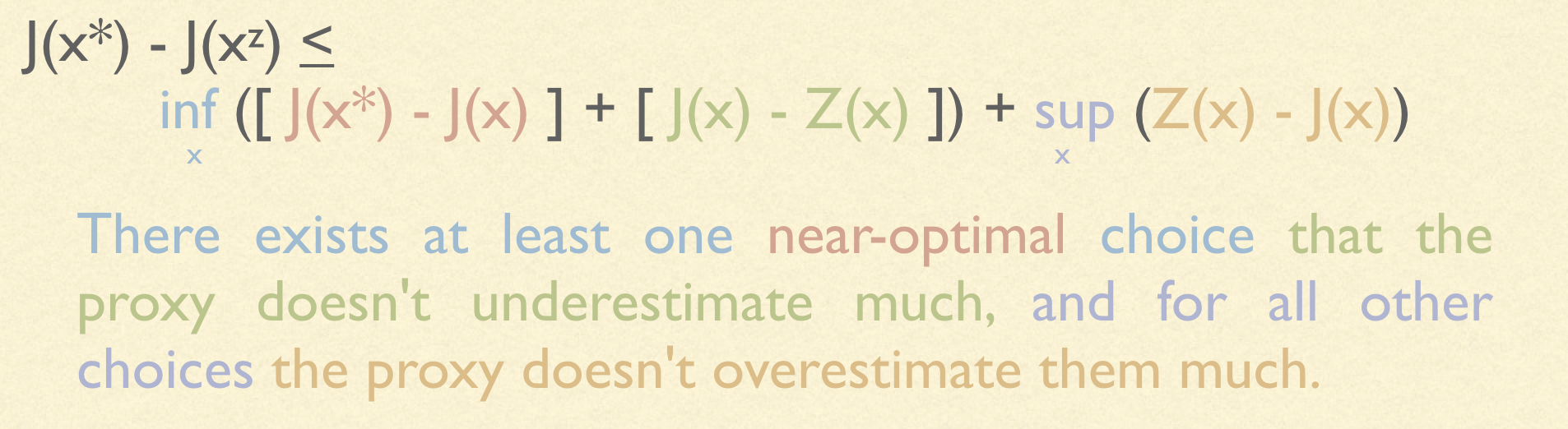
We see an interesting asymmetry between overestimations and underestimations. Underestimations are almost never a problem: all you need is for one good choice to not be underestimated, and the first term becomes small. But overestimations are a huge problem. Thanks to the second term, we could wind up with huge regret if our proxy overestimates even one choice. This tells us something very important. When constructing a proxy objective (e.g. from data), we should intentionally construct it in such a way that large overestimations are impossible, so that the second term remains small.
Pessimism In Offline RL
Okay, let’s bring this back to Offline RL. If you’ll recall, we were trying to answer the question:
What is the best choice of $Q_D^\pi$? How should we estimate the value of a policy from data, in a way that leads to us selecting good policies?
The connection, of course, is that this is precisely the sort of decision problem we discussed in the detour. The space of choices, $X$, is the space of policies, $\Pi$. The objective, $J(\pi)$, is the expected return in the real environment, $Q_M(\pi)$. The proxy objective, $Z(\pi)$, is our estimate of the value of a policy from data, $Q_D(\pi)$. Substituting these values into the regret bound, we see:
The asymmetry between overestimation and underestimation once again appears here; this needs to be reflected in $Q_D$. This motivates the design of pessimistic algorithms, which are constructed to prevent overestimations.
There are many ways to implement pessimism, but in this post we’re going to focus just on the simplest. Let’s return to our very first idea: use the dataset to compute maximum-likelihood estimates of the reward and transition functions, $R_D$ and $P_D$, and use these in the place of $R$ and $P$. Similar to the dynamic programming case, this leads to choosing a $Q_D^\pi$ which obeys Bellman consistency: $Q_D^\pi = R + \gamma P^\pi Q_D^\pi$. Unfortunately, this doesn’t control overestimations at all, so this approach has very large regret. We call this the “naive” approach. It turns out that by simply subtracting a penalty, denoted $K_D$, from Bellman consistency, we can define a $Q_D^\pi$ which is guaranteed to never overestimate at all: $Q_D^\pi = R + \gamma P^\pi Q_D^\pi - K_D$. (Of course, $K_D$ needs to be very carefully chosen – not just any penalty will do! More on this later.) We call this the “lower-bound” approach. By rescaling this penalty by $\alpha$, we can constrain overestimation to be, globally, below any desired value: $Q_D^\pi = R + \gamma P^\pi Q_D^\pi - \alpha K_D$. This gives us a general definition for “pessimistic” approaches, which has both naive and lower-bound as special cases.
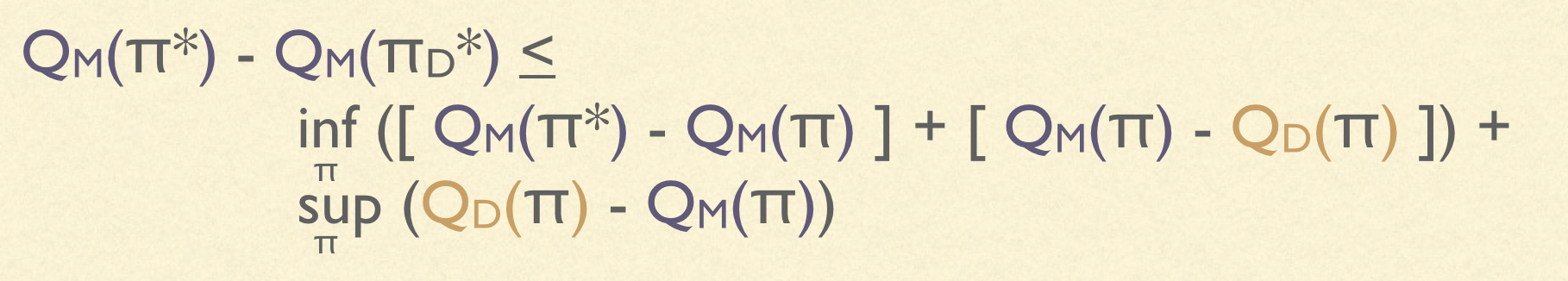
A bit of algebra, and we can derive the regret of a pessimistic algorithm:
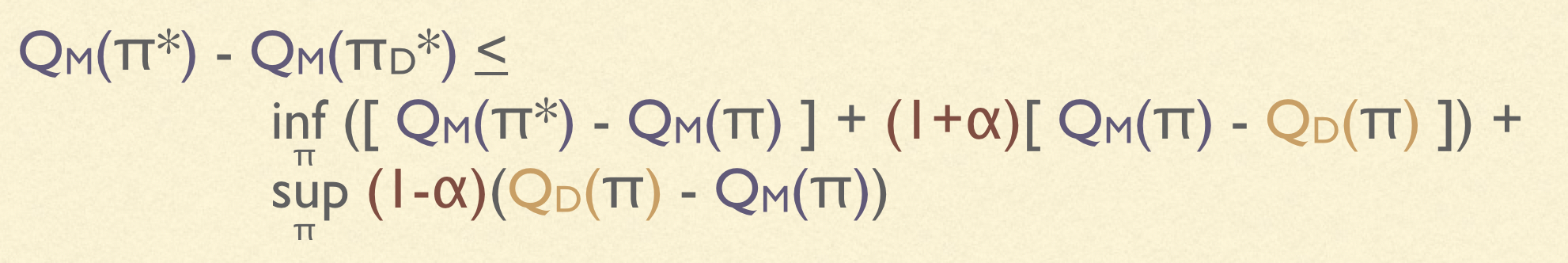
We now see the true importance of pessimism. By increasing $\alpha$, we “shrink” the overestimation, and increase the underestimation by the same amount. But since overestimation lives in a sup term (which is typically large), and underestimation lives in an inf term (which is typically small), this has the net effect of reducing overall regret. Although the optimal value of $\alpha$ is not in general at either 0 or 1, it typically makes sense to set it close to 1, especially in complex environments.
Pessimism Penalties
The final question to be answered is: what is $K_D$? I’m not going to go into the math in detail here, but basically, there are two schools of thought: “uncertainty-aware” and “proximal”.
Uncertainty-aware algorithms follow the intuition, “stick to what we know”. These algorithms choose $K_D$ as an upper-bound on the Bellman residual, e.g. derived from a concentration inequality Hoeffding’s. The policies they learn tend to look similar to the naive policies, but avoiding low-information regions. They converge to the true optimal policy in the limit of a large, diverse dataset.
Proximal algorithms follow the intuition, “copy the empirical policy”. These algorithms choose a $K_D$ which is a divergence from the empirical policy, e.g. total variation between a policy’s action distribution on a state, and the distribution of actions on that state present in the dataset. The policies they learn tend to look similar to imitation-learning policies, which just copy the actions in the dataset; but, they improve on them slightly. Unless the dataset itself is collected according to the optimal policy, proximal algorithms don’t converge to optimal policy, no matter how big the dataset gets.
Surprisingly, proximal algorithms are actually a special case of uncertainty-aware algorithms! We can derive a “relative” uncertainty-aware penalty, which is equivalent to the normal one, but computed relative to the empirical policy. If you take that penalty, and substitute in the “trivial” upper bound to uncertainty of $V_{max}$, what comes out is the proximal $K_D$. Thus, not only are proximal algorithms subsumed by uncertainty-aware algorithms, but the use of a trivial uncertainty means that they are in some sense strictly worse.
However, proximal algorithms do have one key benefit: they can be implemented without computing any form of uncertainty. This is important in deep learning settings, where we don’t yet know how to implement (rigorous) uncertainties. Thus, although proximal algorithms are strictly worse than uncertainty-aware, most recent deep learning approaches have used the proximal technique, simply for its implementability.
All of these theoretical predictions can be readily observed in experiments. Here’s some experiments on a gridworld where we compare the performance of different algorithms on datasets of various sizes.
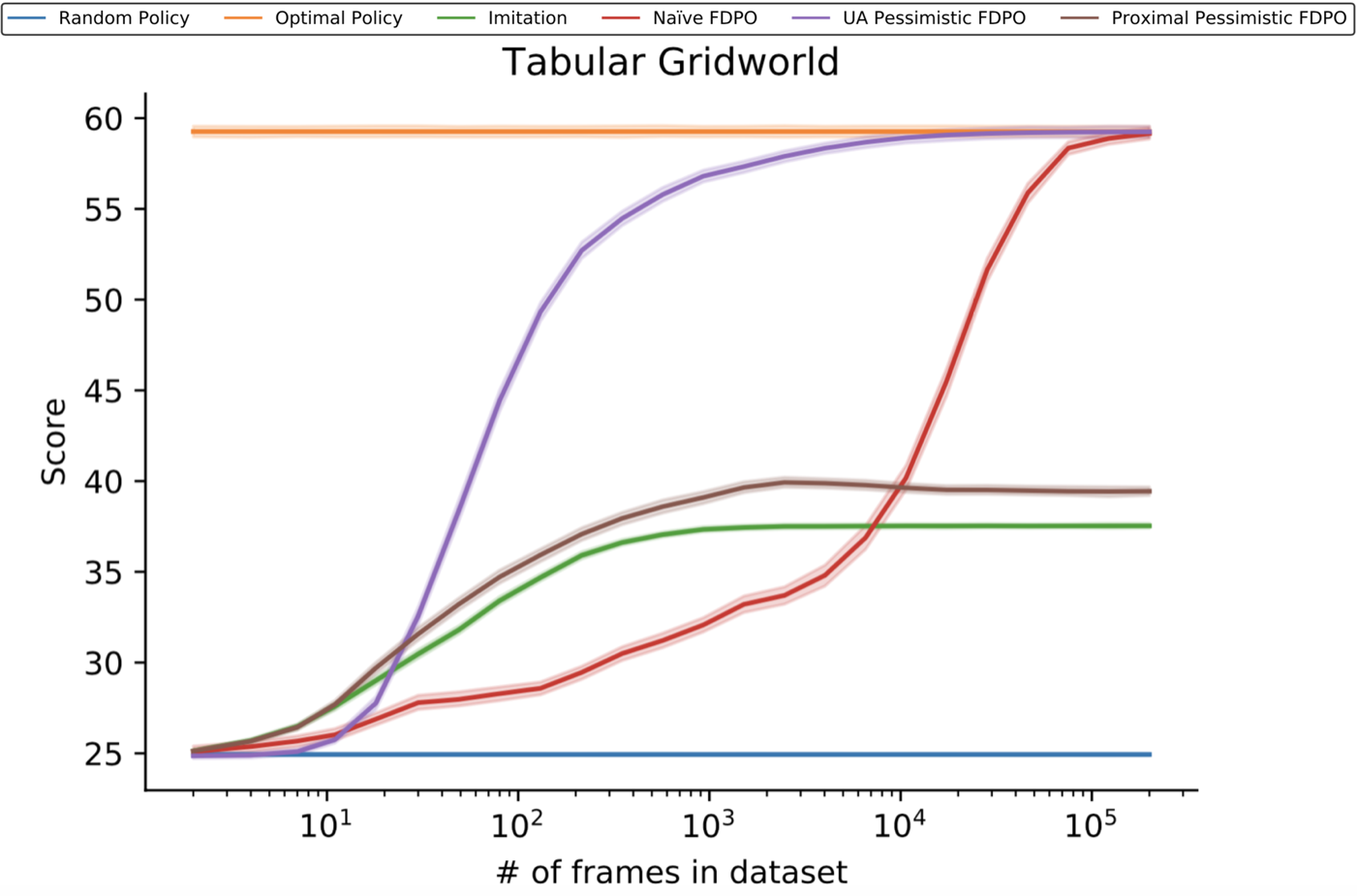
We see the naive approach, the red line, converging to the optimal policy, but very slowly. The UA approach, in purple, converges to the same point, but much more quickly. Unless the dataset is overwhelimngly large, UA pessimism performs far better. The imitation approach, in green, does not converge, since the data-collection policy is constant. And as predicted, the proximal approach, in brown, follows the same trend, but is able to improve on it slightly.
Another set of experiments tests how the diversity of the dataset impacts the suboptimality of various algorithms. The x-axis here corresponds to the $\epsilon$ in an $\epsilon$-greedy data collection policy. On the left, we see fully-random data collection; on the right, fully-optimal. All datasets are the same size, however.
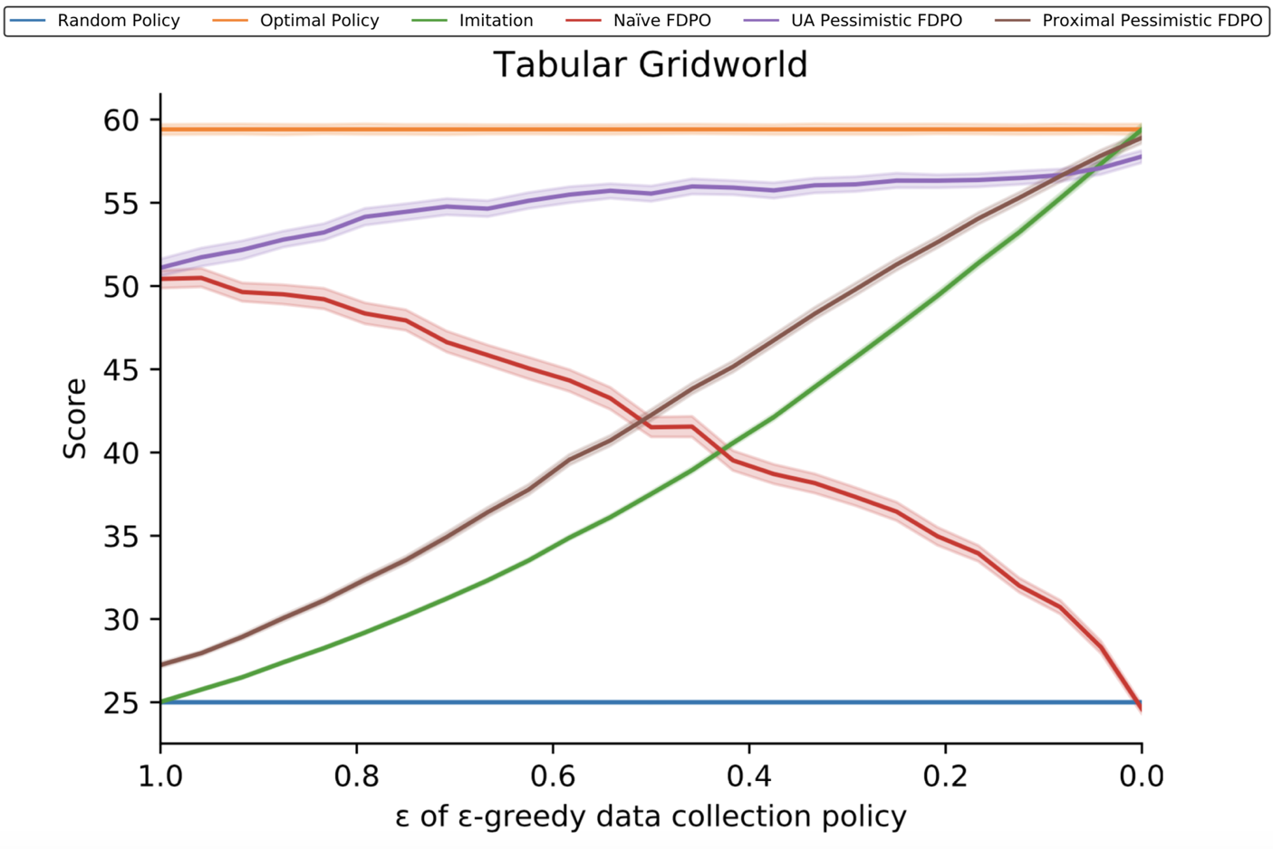
We see the naive approach perform well when data is collected randomly, but poorly when it is collected deterministically – even though in the latter case, all data comes from an optimal policy! This perfectly matches our theoretical prediction that the regret should be controlled mainly by the supremum of overestimaton error. When data is collected stochastically, we get a little information about every policy, so no policy is overestimated much. But the more deteriministically it is collected, the more information we have on the optimal policy, and thus the more likely we are to overestimate some other policy greatly. The other approaches all also clearly match the theory: imitation is better when the collection policy is closer to optimal, proximal algorithms show a slight improvement to imitation, and UA algorithms are good everywhere.
We see similar results on experiments in a deep learning setting, in this case using MinAtar as the testbed:
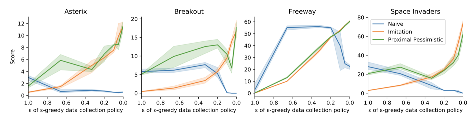
These experiments only test proximal pessimism, because of the aforementioned issue around implementing UA algorithms in deep learning. We see basically the same trends as in the tabular case, if a bit less cleanly.
Conclusion
And that’s all! Let’s finish up with a little recap. TLDR:
Offline RL is about choosing a policy, $\pi_D^{\ast}$, which is near-optimal. We can reduce this to defining $Q_D^\pi$, then taking the argmax $π$. As a proxy objective, a good $Q_D^\pi$ needs to avoid overestimation. We can implement this with penalized Bellman iteration. Penalties can be uncertainty-aware or proximal. Uncertainty-aware is better, but proximal is easier to implement.
If you’d like to learn more, check out my latest paper.
Thanks for reading. Follow me on Substack for more writing, or hit me up on Twitter @jacobmbuckman with any feedback or questions!