This post is the first of a series; click here for the next post.

Click here to skip the intro and dive right in!

Introduction

What is this? Who are you?

I’m Jacob, a Google AI Resident. When I started the residency program in the summer of 2017, I had a lot of experience programming, and a good understanding of machine learning, but I had never used Tensorflow before. I figured that given my background I’d be able to pick it up quickly. To my surprise, the learning curve was fairly steep, and even months into the residency, I would occasionally find myself confused about how to turn ideas into Tensorflow code. I’m writing this blog post as a message-in-a-bottle to my former self: it’s the introduction that I wish I had been given before starting on my journey. Hopefully, it will also be a helpful resource for others.

What was missing?

In the three years since its release, Tensorflow has cemented itself as a cornerstone of the deep learning ecosystem. However, it can be non-intuitive for beginners, especially compared to define-by-run¹ neural network libraries like PyTorch or DyNet.

Many introductory Tensorflow tutorials exist, for doing everything from linear regression, to classifying MNIST, to machine translation. These concrete, practical guides are great resources for getting Tensorflow projects up and running, and can serve as jumping-off points for similar projects. But for the people who are working on applications for which a good tutorial does not exist, or who want to do something totally off the beaten path (as is common in research), Tensorflow can definitely feel frustrating at first.

This post is my attempt to fill this gap. Rather than focusing on a specific task, I take a more general approach, and explain the fundamental abstractions underpinning Tensorflow. With a good grasp of these concepts, deep learning with Tensorflow becomes intuitive and straightforward.

Target Audience

This tutorial is intended for people who already have some experience with both programming and machine learning, and want to pick up Tensorflow. For example: a computer science student who wants to use Tensorflow in the final project of her ML class; a software engineer who has just been assigned to a project that involves deep learning; or a bewildered new Google AI Resident (shout-out to past Jacob). If you’d like a refresher on the basics, here are some resources. Otherwise: let’s get started!

Understanding Tensorflow

Tensorflow Is Not A Normal Python Library

Most Python libraries are written to be natural extensions of Python. When you import a library, what you get is a set of variables, functions, and classes, that augment and complement your “toolbox” of code. When using them, you have a certain set of expectations about how they behave. In my opinion, when it comes to Tensorflow, you should throw all that away. It’s fundamentally the wrong way to think about what Tensorflow is and how it interacts with the rest of your code.

A metaphor for the relationship between Python and Tensorflow is the relationship between Javascript and HTML. Javascript is a fully-featured programming language that can do all sorts of wonderful things. HTML is a framework for representing a certain type of useful computational abstraction (in this case, content that can be rendered by a web browser). The role of Javascript in an interactive webpage is to assemble the HTML object that the browser sees, and then interact with it when necessary by updating it to new HTML.

Similarly to HTML, Tensorflow is a framework for representing a certain type of computational abstraction (known as “computation graphs”). When we manipulate Tensorflow with Python, the first thing we do with our Python code is assemble the computation graph. Once that is done, the second thing we do is to interact with it (using Tensorflow’s “sessions”). But it’s important to keep in mind that the computation graph does not live inside of your variables; it lives in the global namespace. As Shakespeare once said: “All the RAM’s a stage, and all the variables are merely pointers.”

First Key Abstraction: The Computation Graph

In browsing the Tensorflow documentation, you’ve probably found oblique references to “graphs” and “nodes”. If you’re a particularly savvy browser, you may have even discovered this page, which covers the content I’m about to explain in a much more accurate and technical fashion. This section is a high-level walkthrough that captures the important intuition, while sacrificing some technical details.

So: what is a computation graph? Essentially, it’s a global data structure: a directed graph that captures instructions about how to calculate things.

Let’s walk through an example of how to build one. In the following figures, the top half is the code we ran and its output, and the bottom half is the resulting computation graph.

import tensorflow as tf

Graph:

Predictably, just importing Tensorflow does not give us an interesting computation graph. Just a lonely, empty global variable. But what about when we call a Tensorflow operation?

Code:

import tensorflow as tf
two_node = tf.constant(2)
print two_node

Output:

Tensor("Const:0", shape=(), dtype=int32)

Graph:

Would you look at that! We got ourselves a node. It contains the constant 2. Shocking, I know, coming from a function called tf.constant. When we print the variable, we see that it returns a tf.Tensor object, which is a pointer to the node that we just created. To emphasize this, here’s another example:

Code:

import tensorflow as tf
two_node = tf.constant(2)
another_two_node = tf.constant(2)
two_node = tf.constant(2)
tf.constant(3)

Graph:

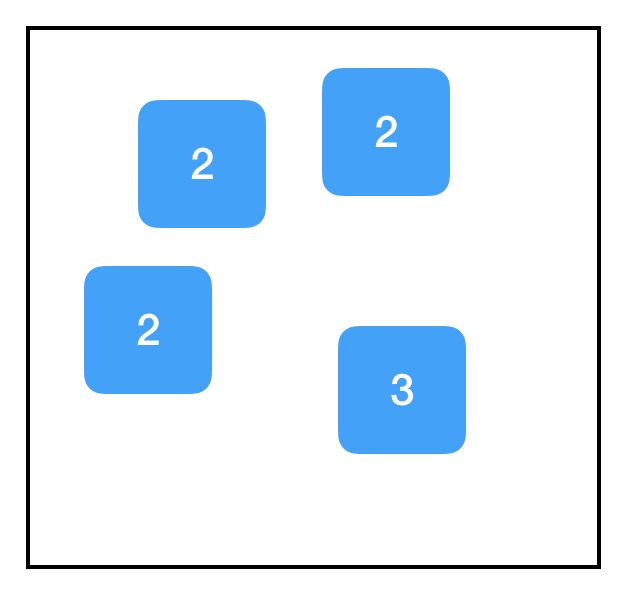
Every time we call tf.constant, we create a new node in the graph. This is true even if the node is functionally identical to an existing node, even if we re-assign a node to the same variable, or even if we don’t assign it to a variable at all.

In contrast, if you make a new variable and set it equal to an existing node, you are just copying the pointer to that node and nothing is added to the graph:

Code:

import tensorflow as tf
two_node = tf.constant(2)
another_pointer_at_two_node = two_node
two_node = None
print two_node
print another_pointer_at_two_node

Output:

None
Tensor("Const:0", shape=(), dtype=int32)

Graph:

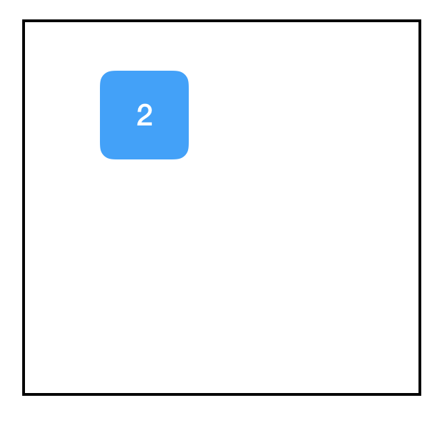
Okay, let’s liven things up a bit:

Code:

import tensorflow as tf
two_node = tf.constant(2)
three_node = tf.constant(3)
sum_node = two_node + three_node ## equivalent to tf.add(two_node, three_node)

Graph:

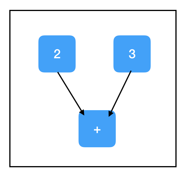
Now we’re talking - that’s a bona-fide computational graph we got there! Notice that the + operation is overloaded in Tensorflow, so adding two tensors together adds a node to the graph, even though it doesn’t seem like a Tensorflow operation on the surface.

Okay, so two_node points to a node containing 2, three_node points to a node containing 3, and sum_node points to a node containing…+? What’s up with that? Shouldn’t it contain 5?

As it turns out, no. Computational graphs contain only the steps of computation; they do not contain the results. At least…not yet!

Second Key Abstraction: The Session

If there were March Madness for misunderstood TensorFlow abstractions, the session would be the #1 seed every year. It has that dubious honor due to being both unintuitively named and universally present – nearly every Tensorflow program explicitly invokes tf.Session() at least once.

The role of the session is to handle the memory allocation and optimization that allows us to actually perform the computations specified by a graph. You can think of the computation graph as a “template” for the computations we want to do: it lays out all the steps. In order to make use of the graph, we also need to make a session, which allows us to actually do things; for example, going through the template node-by-node to allocate a bunch of memory for storing computation outputs. In order to do any computation with Tensorflow, you need both a graph and a session.

The session contains a pointer to the global graph, which is constantly updated with pointers to all nodes. That means it doesn’t really matter whether you create the session before or after you create the nodes. ²

After creating your session object, you can use sess.run(node) to return the value of a node, and Tensorflow performs all computations necessary to determine that value.

Code:

import tensorflow as tf
two_node = tf.constant(2)
three_node = tf.constant(3)
sum_node = two_node + three_node
sess = tf.Session()
print sess.run(sum_node)

Output:

5

Graph:

Wonderful! We can also pass a list, sess.run([node1, node2,...]), and have it return multiple outputs:

Code:

import tensorflow as tf
two_node = tf.constant(2)
three_node = tf.constant(3)
sum_node = two_node + three_node
sess = tf.Session()
print sess.run([two_node, sum_node])

Output:

[2, 5]

Graph:

In general, sess.run() calls tend to be one of the biggest TensorFlow bottlenecks, so the fewer times you call it, the better. Whenever possible, return multiple items in a single sess.run() call instead of making multiple calls.

Placeholders & feed_dict

The computations we’ve done so far have been boring: there is no opportunity to pass in input, so they always output the same thing. A more worthwhile application might involve constructing a computation graph that takes in input, processes it in some (consistent) way, and returns an output.

The most straightforward way to do this is with placeholders. A placeholder is a type of node that is designed to accept external input.

Code:

import tensorflow as tf
input_placeholder = tf.placeholder(tf.int32)
sess = tf.Session()
print sess.run(input_placeholder)

Output:

Traceback (most recent call last):
...
InvalidArgumentError (see above for traceback): You must feed a value for placeholder tensor 'Placeholder' with dtype int32
	 [[Node: Placeholder = Placeholder[dtype=DT_INT32, shape=<unknown>, _device="/job:localhost/replica:0/task:0/device:CPU:0"]()]]

Graph:

…is a terrible example, since it throws an exception. Placeholders expect to be given a value. We didn’t supply one, so Tensorflow crashed.

To provide a value, we use the feed_dict attribute of sess.run().

Code:

import tensorflow as tf
input_placeholder = tf.placeholder(tf.int32)
sess = tf.Session()
print sess.run(input_placeholder, feed_dict={input_placeholder: 2})

Output:

2

Graph:

Much better. Notice the format of the dict passed into feed_dict. The keys should be variables corresponding to placeholder nodes from the graph (which, as discussed earlier, really means pointers to placeholder nodes in the graph). The corresponding values are the data elements to assign to each placeholder – typically scalars or Numpy arrays.

Third Key Abstraction: Computation Paths

Let’s try another example involving placeholders:

Code:

import tensorflow as tf
input_placeholder = tf.placeholder(tf.int32)
three_node = tf.constant(3)
sum_node = input_placeholder + three_node
sess = tf.Session()
print sess.run(three_node)
print sess.run(sum_node)

Output:

3
Traceback (most recent call last):
...
InvalidArgumentError (see above for traceback): You must feed a value for placeholder tensor 'Placeholder_2' with dtype int32
	 [[Node: Placeholder_2 = Placeholder[dtype=DT_INT32, shape=<unknown>, _device="/job:localhost/replica:0/task:0/device:CPU:0"]()]]

Graph:

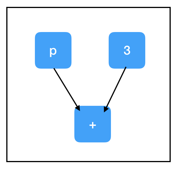
Why does the second call to sess.run() fail? And why does it raise an error related to input_placeholder, even though we are not evaluating input_placeholder? The answer lies in the final key Tensorflow abstraction: computation paths. Luckily, this one is very intuitive.

When we call sess.run() on a node that is dependent on other nodes in the graph, we need to compute the values of those nodes, too. And if those nodes have dependencies, we need to calculate those values (and so on and so on…) until we reach the “top” of the computation graph where nodes have no predecessors.

Consider the computation path of sum_node:

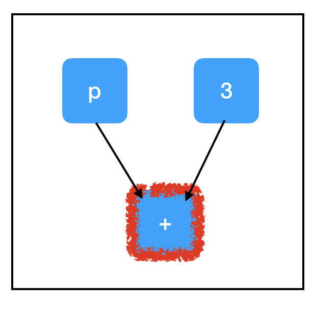
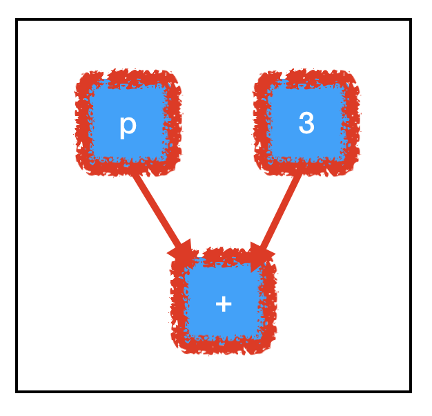
All three nodes need to be evaluated to compute the value of sum_node. Crucially, this includes our un-filled placeholder and explains the exception!

In contrast, consider the computation path of three_node:

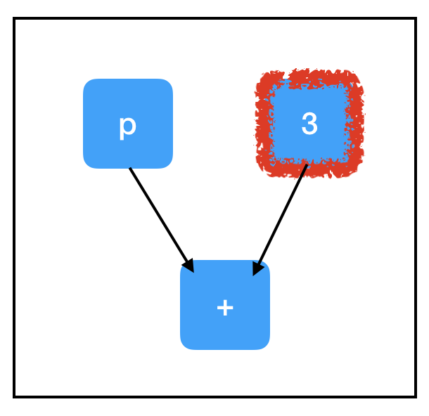
Due to the graph structure, we don’t need to compute all of the nodes in order to evaluate the one we want! Because we don’t need to evaluate placeholder_node to evaluate three_node, running sess.run(three_node) doesn’t raise an exception.

The fact that Tensorflow automatically routes computation only through nodes that are necessary is a huge strength of the framework. It saves a lot of runtime on calls if the graph is very big and has many nodes that are not necessary. It allows us to construct large, “multi-purpose” graphs, which use a single, shared set of core nodes to do different things depending on which computation path is taken. For almost every application, it’s important to think about sess.run() calls in terms of the computation path taken.

Variables & Side Effects

So far, we’ve seen two types of “no-ancestor” nodes: tf.constant, which is the same for every run, and tf.placeholder, which is different for every run. There’s a third case that we often want to consider: a node which generally has the same value between runs, but can also be updated to have a new value. That’s where variables come in.

Understanding variables is essential to doing deep learning with Tensorflow, because the parameters of your model fall into this category. During training, you want to update your parameters at every step, via gradient descent; but during evaluation, you want to keep your parameters fixed, and pass a bunch of different test-set inputs into the model. More than likely, all of your model’s trainable parameters will be implemented as variables.

To create variables, use tf.get_variable().³ The first two arguments to tf.get_variable() are required; the rest are optional. They are tf.get_variable(name, shape). name is a string which uniquely identifies this variable object. It must be unique relative to the global graph, so be careful to keep track of all names you have used to ensure there are no duplicates.⁴ shape is an array of integers corresponding to the shape of a tensor; the syntax of this is intuitive – just one integer per dimension, in order. For example, a 3x8 matrix would have shape [3, 8]. To create a scalar, use an empty list as your shape: [].

Code:

import tensorflow as tf
count_variable = tf.get_variable("count", [])
sess = tf.Session()
print sess.run(count_variable)

Output:

Traceback (most recent call last):
...
tensorflow.python.framework.errors_impl.FailedPreconditionError: Attempting to use uninitialized value count
	 [[Node: _retval_count_0_0 = _Retval[T=DT_FLOAT, index=0, _device="/job:localhost/replica:0/task:0/device:CPU:0"](count)]]

Graph:

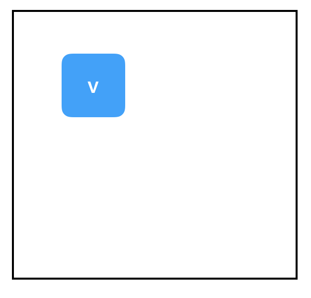
Alas, another exception. When a variable node is first created, it basically stores “null”, and any attempts to evaluate it will result in this exception. We can only evaluate a variable after putting a value into it first. There are two main ways to put a value into a variable: initializers and tf.assign(). Let’s look at tf.assign() first:

Code:

import tensorflow as tf
count_variable = tf.get_variable("count", [])
zero_node = tf.constant(0.)
assign_node = tf.assign(count_variable, zero_node)
sess = tf.Session()
sess.run(assign_node)
print sess.run(count_variable)

Output:

0

Graph:

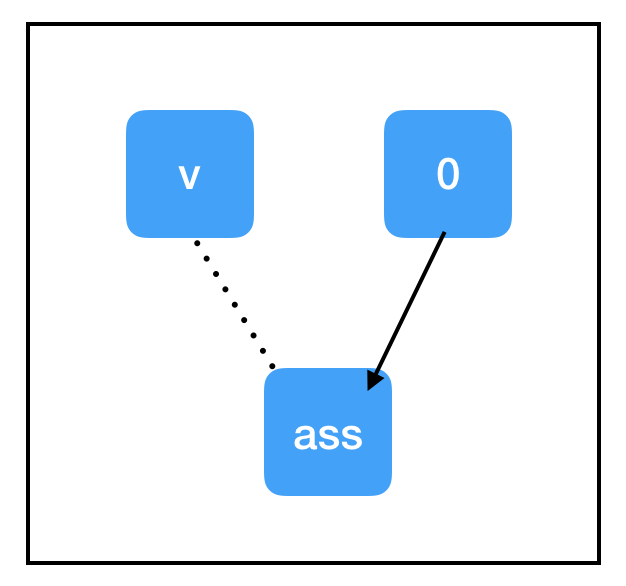
tf.assign(target, value) is a node that has some unique properties compared to nodes we’ve seen so far:

• Identity operation. tf.assign(target, value) does not do any interesting computations, it is always just equal to value.
• Side effects. When computation “flows” through assign_node, side effects happen to other things in the graph. In this case, the side effect is to replace the value of count_variable with the value stored in zero_node.
• Non-dependent edges. Even though the count_variable node and the assign_node are connected in the graph, neither is dependent on the other. This means computation will not flow back through that edge when evaluating either node. However, assign_node is dependent on zero_node; it needs to know what to assign.

“Side effect” nodes underpin most of the Tensorflow deep learning workflow, so make sure you really understand what’s going on here. When we call sess.run(assign_node), the computation path goes through assign_node and zero_node.

Graph:

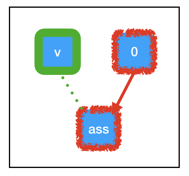
As computation flows through any node in the graph, it also enacts any side effects controlled by that node, shown in green. Due to the particular side effects of tf.assign, the memory associated with count_variable (which was previously “null”) is now permanently set to equal 0. This means that when we next call sess.run(count_variable), we don’t throw any exceptions. Instead, we get a value of 0. Success!

Next, let’s look at initializers:

Code:

import tensorflow as tf
const_init_node = tf.constant_initializer(0.)
count_variable = tf.get_variable("count", [], initializer=const_init_node)
sess = tf.Session()
print sess.run([count_variable])

Output:

Traceback (most recent call last):
...
tensorflow.python.framework.errors_impl.FailedPreconditionError: Attempting to use uninitialized value count
	 [[Node: _retval_count_0_0 = _Retval[T=DT_FLOAT, index=0, _device="/job:localhost/replica:0/task:0/device:CPU:0"](count)]]

Graph:

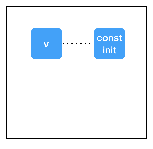
Okay, what happened here? Why didn’t the initializer work?

The answer lies in the split between sessions and graphs. We’ve set the initializer property of get_variable to point at our const_init_node, but that just added a new connection between nodes in the graph. We haven’t done anything about the root of the exception: the memory associated with the variable node (which is stored in the session, not the graph!) is still set to “null”. We need the session to tell the const_init_node to actually update the variable.

Code:

import tensorflow as tf
const_init_node = tf.constant_initializer(0.)
count_variable = tf.get_variable("count", [], initializer=const_init_node)
init = tf.global_variables_initializer()
sess = tf.Session()
sess.run(init)
print sess.run(count_variable)

Output:

0.

Graph:

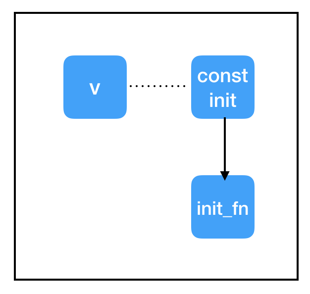
To do this, we added another, special node: init = tf.global_variables_initializer(). Similarly to tf.assign(), this is a node with side effects. In contrast to tf.assign(), we don’t actually need to specify what its inputs are! tf.global_variables_initializer() will look at the global graph at the moment of its creation and automatically add dependencies to every tf.initializer in the graph. When we then evaluate it with sess.run(init), it goes to each of the initializers and tells them to do their thang, initializing the variables and allowing us to run sess.run(count_variable) without an error.

Variable Sharing

You may encounter Tensorflow code with variable sharing, which involves creating a scope and setting “reuse=True”. I strongly recommend that you don’t use this in your own code. If you want to use a single variable in multiple places, simply keep track of your pointer to that variable’s node programmatically, and re-use it when you need to. In other words, you should have only a single call of tf.get_variable() for each parameter you intend to store in memory.

Optimizers

At last: on to the actual deep learning! If you’re still with me, the remaining concepts should be extremely straightforward.

In deep learning, the typical “inner loop” of training is as follows:

1. Get an input and true_output
2. Compute a “guess” based on the input and your parameters
3. Compute a “loss” based on the difference between your guess and the true_output
4. Update the parameters according to the gradient of the loss

Let’s put together a quick script for a toy linear regression problem:

Code:

import tensorflow as tf

### build the graph
## first set up the parameters
m = tf.get_variable("m", [], initializer=tf.constant_initializer(0.))
b = tf.get_variable("b", [], initializer=tf.constant_initializer(0.))
init = tf.global_variables_initializer()

## then set up the computations
input_placeholder = tf.placeholder(tf.float32)
output_placeholder = tf.placeholder(tf.float32)

x = input_placeholder
y = output_placeholder
y_guess = m * x + b

loss = tf.square(y - y_guess)

## finally, set up the optimizer and minimization node
optimizer = tf.train.GradientDescentOptimizer(1e-3)
train_op = optimizer.minimize(loss)

### start the session
sess = tf.Session()
sess.run(init)

### perform the training loop
import random

## set up problem
true_m = random.random()
true_b = random.random()

for update_i in range(100000):
  ## (1) get the input and output
  input_data = random.random()
  output_data = true_m * input_data + true_b

  ## (2), (3), and (4) all take place within a single call to sess.run()!
  _loss, _ = sess.run([loss, train_op], feed_dict={input_placeholder: input_data, output_placeholder: output_data})
  print update_i, _loss

### finally, print out the values we learned for our two variables
print "True parameters:     m=%.4f, b=%.4f" % (true_m, true_b)
print "Learned parameters:  m=%.4f, b=%.4f" % tuple(sess.run([m, b]))

Output:

0 2.3205383
1 0.5792742
2 1.55254
3 1.5733259
4 0.6435648
5 2.4061265
6 1.0746256
7 2.1998715
8 1.6775116
9 1.6462423
10 2.441034
...
99990 2.9878322e-12
99991 5.158629e-11
99992 4.53646e-11
99993 9.422685e-12
99994 3.991829e-11
99995 1.134115e-11
99996 4.9467985e-11
99997 1.3219648e-11
99998 5.684342e-14
99999 3.007017e-11
True parameters:     m=0.3519, b=0.3242
Learned parameters:  m=0.3519, b=0.3242

As you can see, the loss goes down to basically nothing, and we wind up with a really good estimate of the true parameters. Hopefully, the only part of the code that is new to you is this segment:

## finally, set up the optimizer and minimization node
optimizer = tf.train.GradientDescentOptimizer(1e-3)
train_op = optimizer.minimize(loss)

But, now that you have a good understanding of the concepts underlying Tensorflow, this code is easy to explain! The first line, optimizer = tf.train.GradientDescentOptimizer(1e-3), is not adding a node to the graph. It is simply creating a Python object that has useful helper functions. The second line, train_op = optimizer.minimize(loss), is adding a node to the graph, and storing a pointer to it in variable train_op. The train_op node has no output, but has a very complicated side effect:

train_op traces back through the computation path of its input, loss, looking for variable nodes. For each variable node it finds, it computes the gradient of the loss with respect to that variable. Then, it computes a new value for that variable: the current value minus the gradient times the learning rate. Finally, it performs an assign operation to update the value of the variable.

So essentially, when we call sess.run(train_op), it does a step of gradient descent on all of our variables for us. Of course, we also need to fill in the input and output placeholders with our feed_dict, and we also want to print the loss, because it’s handy for debugging.

Debugging with tf.Print

As you start doing more complicated things with Tensorflow, you’re going to want to debug. In general, it’s quite hard to inspect what’s going on inside a computation graph. You can’t use a regular Python print statement, because you never have access to the values you want to print – they are locked away inside the sess.run() call. To elaborate, suppose you want to inspect an intermediate value of a computation. Before the sess.run() call, the intermediate values do not exist yet. But when the sess.run() call returns, the intermediate values are gone!

Let’s look at a simple example.

Code:

import tensorflow as tf
two_node = tf.constant(2)
three_node = tf.constant(3)
sum_node = two_node + three_node
sess = tf.Session()
print sess.run(sum_node)

Output:

5

This lets us see our overall answer, 5. But what if we want to inspect the intermediate values, two_node and three_node? One way to inspect the intermediate values is to add a return argument to sess.run() that points at each of the intermediate nodes you want to inspect, and then, after it has been returned, print it.

Code:

import tensorflow as tf
two_node = tf.constant(2)
three_node = tf.constant(3)
sum_node = two_node + three_node
sess = tf.Session()
answer, inspection = sess.run([sum_node, [two_node, three_node]])
print inspection
print answer

Output:

[2, 3]
5

This often works well, but as code becomes more complex, it can be a bit awkward. A more convenient approach is to use a tf.Print statement. Confusingly, tf.Print is actually a type of Tensorflow node, which has both output and side effects! It has two required arguments: a node to copy, and a list of things to print. The “node to copy” can be any node in the graph; tf.Print is an identity operation with respect to its “node to copy”, meaning that it outputs an exact copy of its input. But, it also prints all the current values in the “list of things to print” as a side effect.⁵

Code:

import tensorflow as tf
two_node = tf.constant(2)
three_node = tf.constant(3)
sum_node = two_node + three_node
print_sum_node = tf.Print(sum_node, [two_node, three_node])
sess = tf.Session()
print sess.run(print_sum_node)

Output:

[2][3]
5

Graph:

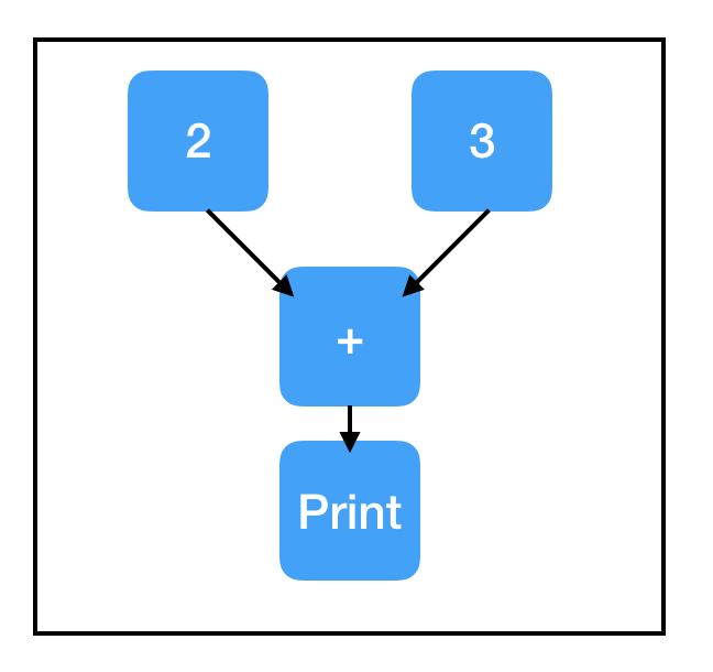
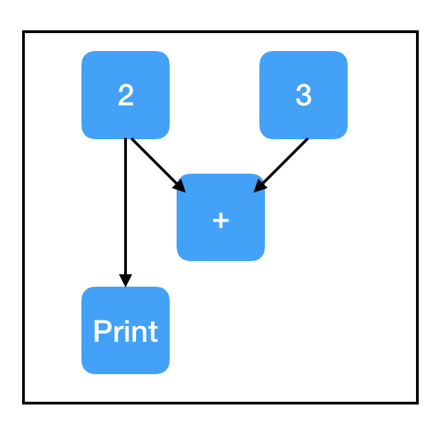
One important, somewhat-subtle point about tf.Print: printing is a side effect. Like all other side effects, printing only occurs if the computation flows through the tf.Print node. If the tf.Print node is not in the path of the computation, nothing will print. In particular, even if the original node that your tf.Print node is copying is on the computation path, the tf.Print node itself might not be. Watch out for this issue! When it strikes (and it eventually will), it can be incredibly frustrating if you aren’t specifically looking for it. As a general rule, try to always create your tf.Print node immediately after creating the node that it copies.

Code:

import tensorflow as tf
two_node = tf.constant(2)
three_node = tf.constant(3)
sum_node = two_node + three_node
### this new copy of two_node is not on the computation path, so nothing prints!
print_two_node = tf.Print(two_node, [two_node, three_node, sum_node])
sess = tf.Session()
print sess.run(sum_node)

Output:

5

Graph:

Here is a great resource which provides additional practical debugging advice.

Conclusion

Hopefully this post helped you get a better intuition for what Tensorflow is, how it works, and how to use it. At the end of the day, the concepts presented here are fundamental to all Tensorflow programs, but this is only scratching the surface. In your Tensorflow adventures, you will likely encounter all sorts of other fun things that you want to use: conditionals, iteration, distributed Tensorflow, variable scopes, saving & loading models, multi-graph, multi-session, and multi-core, data-loader queues, and much more. Many of these topics I will cover in future posts. But if you build on the ideas you learned here with the official documentation, some code examples, and just a pinch of deep learning magic, I’m sure you’ll be able to figure it out!

For more detail on how these abstractions are implemented in Tensorflow, and how to interact with them, take a look at my post on inspecting computational graphs.

Please give me feedback in the comments (or via email) if anything discussed in this guide was unclear. And if you enjoyed this post, let me know what I should cover next!

Happy training!

This post is the first of a series; click here for the next post.

Thanks for reading. Follow me on Substack for more writing, or hit me up on Twitter @jacobmbuckman with any feedback or questions!

Many thanks to Kathryn Rough, Katherine Lee, Sara Hooker, and Ludwig Schubert for all of their help and feedback when writing this post.