Three Paradigms of Reinforcement Learning

by Carles Gelada and Jacob Buckman

Many researchers believe that model-based reinforcement learning (MBRL) is more sample-efficient that model-free reinforcement learning (MFRL). However, at a fundamental level, this claim is false. A more nuanced analysis shows that it can be the case that MBRL approaches are more sample-efficient than MFRL approaches when using neural networks, but only on certain tasks. Furthermore, we believe that model-based RL is only the beginning. Another family of algorithms, homomorphism-based reinforcement learning (HBRL), may hold the potential to provide further gains in sample-efficiency on tasks with high levels of irrelevant information, like visual distractors. In this post, we provide an intuitive justification for these ideas.

Equivalence Between Model-based and Model-free RL

“Model-based methods are more sample efficient that model-free methods.” This oft-repeated maxim has reared its head in almost every model-based RL paper in recent years (including Jacob’s). It’s such common knowledge that nobody even bothers including a citation alongside – the truth of the statement is taken as self-evident. It’s obvious…and yet it is false. In fact, in many cases, the sample-efficiency of the two approaches is identical.

This equivalence between MBRL and MFRL can be seen when comparing the value functions that the two methods learn given a dataset of transitions. The model-free approach is to learn this value function directly, via TD learning. In contrast, the model-based approach is to learn this value function implicitly, by learning a model of the transitions, and then unrolling it; the sum of the discounted rewards gives us the value. Given the same dataset of transitions, each of these two methods will compute an approximation to the true value function; when data is plentiful, both methods will give a near-perfect approximation. The sample efficiency of an algorithm refers to how quickly the approximation error decreases as more and more data becomes available.

These two algorithms appear very different on the surface, and so we might expect that the error decreases at different rates. Yet, as proven in Parr 2008, in tabular and linear settings these two approaches not only have the same rates, but in fact lead to the exact same value functions! The two approaches are equivalent. There is nothing fundamental about the model-based approach that causes it to be more sample-efficient.

And yet, even once this equivalence is known, many researchers still have a powerful intuition that learning a model of the environment is somehow better. We agree! Let’s attempt to further explore this intuition, so we can better understand where it may or may not hold.

The Simpler, the Sample-efficient-er

First, we want to highlight a principle that is core to the arguments on this post, one that will be familiar to anyone who has trained a neural network. On almost any task, the amount of data required to train a neural network to a good performance is more-or-less proportional to the difficulty of the task, as measured by the complexity of the function which corresponds to the “right answer”¹. Training a neural network to predict a constant output for all inputs requires only a handful of data points; accurate classification on MNIST is achieved in the thousands of examples; ImageNET requires millions.

A Motivating Example: City Navigation

Consider the task of navigation in a city, which we pose as an RL problem. At the beginning of each episode a map is generated, and an initial position of the agent and a target are sampled. The state space is a top-down pixel representation of the city’s grid. To get a reward, the agent must travel from the start point to the target point by selecting up, down, left or right actions. Let’s consider what it would take to solve this MDP using both model-free and model-based techniques.

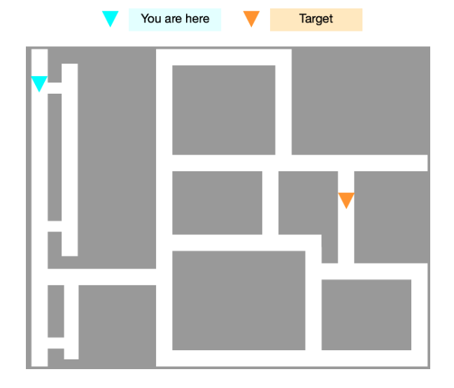
For the model-free approach, we try to learn a value function: a neural net mapping from the state space directly to a value for each action. However, this will be fairly challenging to learn. The city is maze-like, and adding (or removing) a small shortcut, even one far from the agent or the target, could significantly alter the agent’s expected return. Therefore, two similar-seeming states could have dramatically different values. In other words, the value function is a highly complex function of the state. Since this value function is not at all simple, a large amount of data is required to approximate it with a neural network.

The model-based approach is more intuitively close to how a human would understand the task. In this second approach, we train a neural network to approximate the rewards and transitions of the environment. Once an approximate model has been learned, the optimal policy can be extracted via planning (i.e., rollout futures from different actions using the model, and take the action with the highest expected return). From a generalization perspective, the benefits of using the model-based approach on this task are immediately apparent. The simple dynamics (i.e. move the agent in the direction of the action except if there is a wall) result in simple learning objectives for the transition and reward model. Since we are learning a simple function, we will not require very much data to achieve good performance, and will thus be more sample-efficient.

So What Changed?

Why does this argument hold, rather than fall victim to the equivalence described above? The key is neural networks. The equivalence described by Parr (2008) exists only in the tabular and linear settings. When both the true value function and true dynamics are linear functions of the state space, it’s clear that neither is simpler to learn than the other! However, when our state-space is high-dimensional and our function classes are neural networks, the complexity of the function that we choose to learn has a big impact on how many samples it takes to succeed. Any gains or losses in sample-efficiency are intimately tied to generalization behavior.

Furthermore, this interpretation lets us understand which tasks we expect to improve in sample-efficiency when we switch to model-based reinforcement learning. Simply put, in tasks with simple dynamics but complex optimal policies, understanding of the dynamics is a more efficient approach than brute forcing the optimal policy. But crucially, note that this is not true of every task! Consider a modification to the city navigation example, where the agent’s observation space is augmented by GPS navigation directions. This is an example of a task where the optimal policy is simpler than the dynamics; thus, a task where model-free learning would be more sample-efficient.

It’s easy to see intuitively that some MDPs are easier to solve model-based or model-free, but much work remains to understand this distinction rigorously. A recent paper by Dong et al. has begun to formalize this notion, proving that there exist many MDPs for which the policy and Q-function are more complex than the dynamics. Hopefully, future work will continue to build on these ideas, eventually painting a clear picture of how to characterize the difference.

Modeling in a More Realistic Setting

But model-based vs. model-free is only part of the picture. The navigation task above was amenable to model-learning because its dynamics were simple and straightforward. But in the real world, things are typically not so clean. Consider a variant of the same maze task, but rendered more realistically, as though the input pixels were provided by a camera:

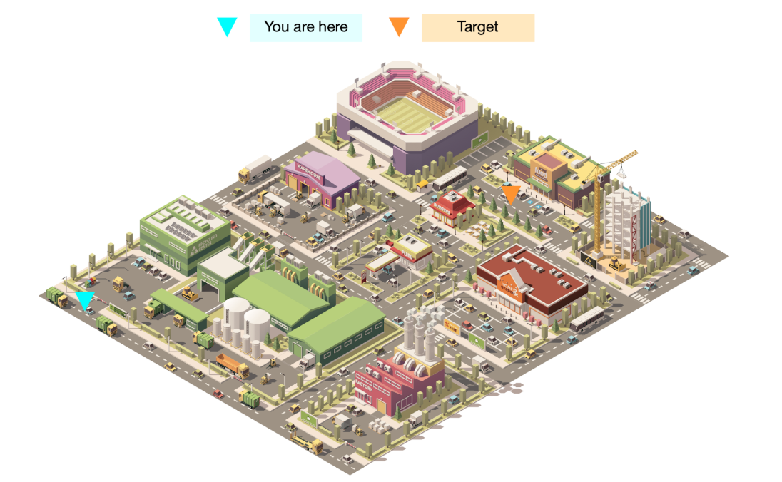
Although the task is fundamentally unchanged, it is far more difficult to learn a dynamics model in this environment. Since the state space is represented by pixels, a prediction of the next state requires that we predict how every single pixel on the screen changes in response to our actions. We need to predict pixel-by-pixel how the smoke floats up from the smokestacks, how the shadows flow across the ground, whether the football team in the stadium scores or not. Even if we could learn such a model (not an easy task for finite-capacity neural networks), we would require an enormous amount of data to generalize well. The real world is extraordinarily complex, and so any algorithm which attempts to model the real world with neural networks will suffer from extraordinarily poor sample efficiency.

Homomorphism-Based RL

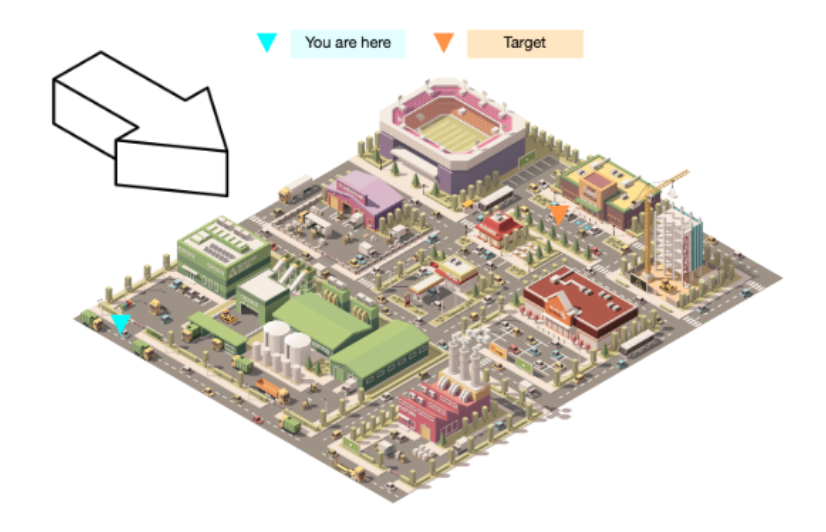
The idea that adding visual complexity greatly increases the difficulty of a problem does not seem to reflect human experience. The visual addition of trees and cars to the navigation problem has not changed your perception of the problem, or your ability to come up with a solution. Even without knowledge of the precise movement of the smoke and shadows, humans still have access to a model of the task. We understand what matters, and we understand the dynamics of the things that matter.

In other words, humans have the ability to intuitively reduce the visually-noisy realistic city grid into an equivalent simplified version. More generally, for almost any task, people are able to project the messy, high-dimensional real world state into a clean, low-dimensional representation. Crucially, these representations contain only the task-relevant features of the original state, and discards all the useless complexity. Any noise, redundancy, etc., is completely absent. In the latent space defined by these representations, the dynamics once again become very simple, and we can easily and sample-efficiently do planning.

We refer to this idea as homomorphism-based RL (HBRL). This represents a third paradigm by which we can design reinforcement learning algorithms. The name “homomorphism” stems from the mathematical interpretation of the learned representation space as a simplified MDP, which is homomorphic (a form of equivalence) to the environment MDP. In tasks with complex value functions and state dynamics, but simple underlying task dynamics, we should expect that homomorphism-based RL will be the most sample-efficient way to learn.

Of course, just as we saw in our earlier discussion of MFRL vs. MBRL, HBRL is not always the best solution. For example, if we are attempting to solve a very simple environment (like the simplified city task from before), HBRL will generally require more data than MBRL, since the algorithm will require many datapoints just to realize that the best latent space is the state space itself. And of course, even in a realistic city environment, GPS directions will still result in model-free learning being more sample efficient than any alternative.

And yet: when it comes to real-world tasks, it’s intuitively clear that the vast majority of them will resemble the realistic city task. The real world is a visually complex place, and “step-by-step” instructions are rarely given. Therefore, we believe that sample-efficient learning in real-world environments is likely to be hugely accelerated by progress in latent-model-based RL.

Homomorphism-Based RL vs. Latent-Space Modeling

If you have been following recent trends in deep reinforcement learning, the idea of “learning an equivalent but simplified latent-space model” might seem familiar to you. Indeed, from a surface-level read, recent works like World Models (Ha et al) and PlaNet (Hafner et al) seem to match our above definition of homomorphism-based RL. However, there is a crucial distinction.

The core idea behind HBRL is that a good representation of the state does not need to include task-irrelevant information. If we force the latent space to encode arbitrary information about the state space – for example, by minimizing a reconstruction loss – we encounter difficulties in environments with complex state spaces (essentially the same difficulties encountered by MBRL). The aforementioned approaches all include either state-reconstruction or next-state-prediction losses, and so they are best characterized as doing MBRL with latent variables, not HBRL.

Previous Work on Homomorphic MDPs

In the last few decades, several works have explored these ideas. Bisimulation, MDP homomorphisms, and state abstraction all proposed sound mathematical foundations to think about what it means for information to be relevant to a task. These research directions led to tabular RL algorithms based on learning state representations through aggregation.

And yet, it’s likely that most readers of this blog have never heard of these papers. That is because, despite being much more algorithmically complex, these methods never showed improvements over simpler approaches. The reason for this deficiency: just as model-based and model-free reinforcement learning are equivalent in the tabular setting, so too are these methods². Since all techniques are fundamentally equivalent, there’s no reason to introduce the added complexity of state abstraction.

But once again, when neural networks are involved, it’s a different story. Since effective generalization becomes key to sample efficiency, there are many environments for which learning a state abstraction is far more sample-efficient than alternative approaches. Specifically, this is the case for environments with large amounts of task-irrelevant information in the state space, such as the realistic city navigation task introduced in the previous section.

Unfortunately, since many of these techniques are closely tied to tabular environments, almost no progress has been made in adapting them to modern deep reinforcement learning settings. We believe this is one of the most promising research avenues in deep reinforcement learning. In our recent ICML paper, we laid the theoretical groundwork for a class of homomorphic RL algorithms that are compatible with neural networks. We formulate the problem of understanding what matters as the problem of learning a neural embedding function for the states of an MDP. Then, understanding the dynamics of what matters corresponds to learning a neural model of the dynamics in the latent space defined by the embedding function. Carles decided to call this framework the “DeepMDP”, but in retrospect, that name is terrible and we wish we had named it something else.

Latent Planning with DeepMDPs

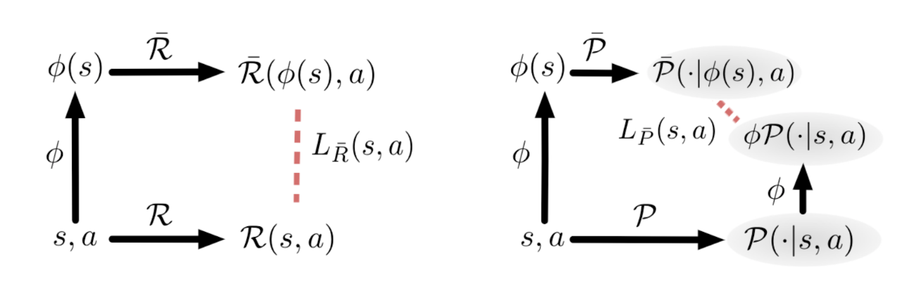
A DeepMDP consists of a set of three functions, each represented by a neural network: an embedding function $\phi : S \rightarrow \bar{S}$ which maps from states to latent representations, a reward function $\bar{\mathcal{R}} : \bar{S} \times A \rightarrow \mathbb{R}$ which maps from latent-states and actions to rewards, and a transition function $\bar{\mathcal{P}} : \bar{S} \times A \rightarrow \bar{S}$ which maps from latent-states and actions to next-latent-states. (These latter two are sometimes collectively referred to as the “latent-space model”.)

Crucially, a DeepMDP is trained by the minimization of two objective functions, one for the reward $L_{\bar{\mathcal{R}}}(s,a)$ and one for the transition $L_{\bar{\mathcal{P}}}(s,a)$. Intuitively, given a state and an action, these functions measure the distance between the outcome of the real reward/transition function, and the outcome of the latent reward/transition function. These objectives are visualized below:

What Guarantees Can We Obtain?

There are two valuable properties that are obtained by minimizing these objectives:

1. The embedding function will only discard task-irrelevant information of the state.
2. The latent-space model and the embedded states of the real MDP follow precisely the same dynamics, meaning the transitions and rewards always align perfectly.

It’s intuitively clear how the second property is satisfied by the minimization of the DeepMDP objectives. Essentially, we are enforcing that the embedding and transition functions commute, and that the states and latent states have the same rewards. In other words, we are enforcing a homomorphism between the environment’s MDP and the DeepMDP.

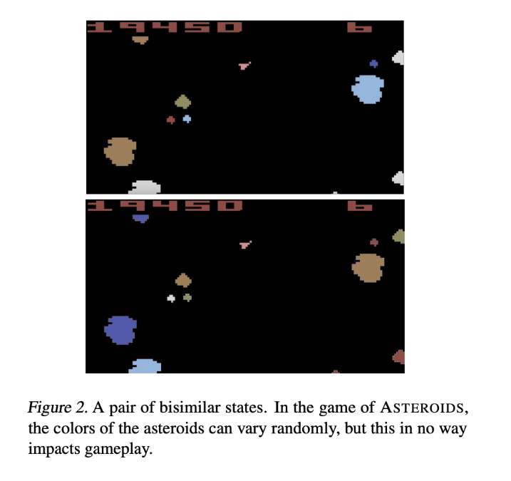
However, it’s much less apparent that property (1) must be satisfied. To show that it is, we analyze the properties of a trained DeepMDP with the help of bisimulation metrics (one of the mathematical foundations for RL representation learning that we mentioned earlier). Bisimulation metrics measure a notion of “behavioral similarity” between any two states. Under these metrics, the distance between two states is small if they possess similar distributions of both immediate and future rewards. Any two states that only differ by visual elements that don’t affect the dynamics of the game (such as the differing asteroid colors in the ASTEROIDS figure below), have bisimulation distance 0. Therefore, our first objective can be understood as learning an embedding function that respects bisimulation: in other words, an embedding function that only collapses states together when the bisimulation distance between them is 0. Somewhat surprisingly, we can mathematically guarantee that this will be the case for any embedding function that is learned by minimizing the DeepMDP objectives.

Global vs. Local Losses

Note that the objectives above are functions; they give us a loss for each state and an action. The MDP contains many states and actions, and in order to apply optimization algorithms, we need to compile these per-state-action losses into a single scalar loss value³. In the paper, we began by studying the minimization of the supremum of all losses over the whole state-action space, which we term the global DeepMDP losses. We proved that when the global DeepMDP losses are minimized, two important things must be true. Firstly, the learned embedding function is guaranteed to respect bisimulation. Secondly, the DeepMDP is guaranteed to be an accurate model of the real environment.

Unfortunately, minimization of the supremum is not possible in practice. Neural networks are trained using an expectation of states and actions, sampled from a distribution. Therefore, we also studied guarantees provided by the minimization of the local DeepMDP losses, which are computed by taking the expectation of the loss functions under a state-action distribution. (So-named because they measure the loss “locally” with respect to said distribution.) Just as in the global case, we proved that when the local DeepMDP losses are minimized, the DeepMDP is guaranteed to be an accurate model of the real environment.

Unfortunately, there isn’t a connection between the local losses and bisimulation metrics. This is because classic bisimulation inherently depends on the entire state-action space. We speculate that there exist local variants of bisimulation metrics, which will allow us to fully understand the representations learned by DeepMDPs (work in progress).

Empirical Results

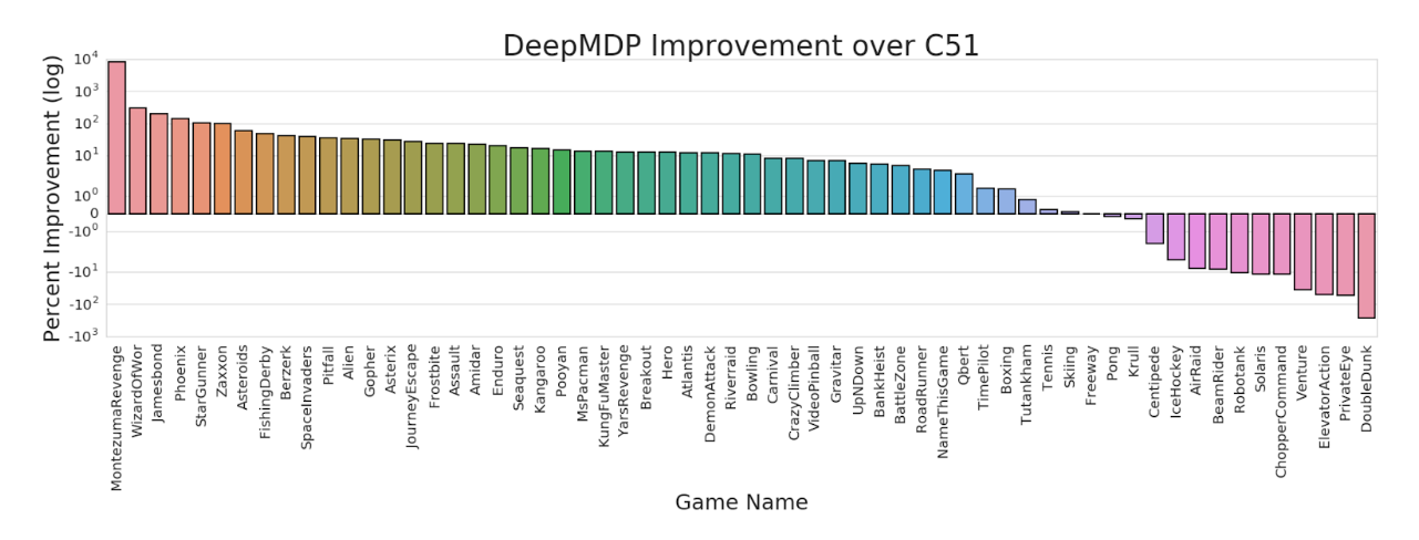
Since DeepMDPs are fully compatible with neural networks, it is only natural that we test them out on standard deep RL benchmarks. Thus far, we have only explored the representation-learning aspect of DeepMDPs. To do so, we applied a simple modification to a standard Atari 2600 agent: we selected an intermediate layer of the Q-function’s neural network to be the DeepMDP latent space, and added a reward and transition model which were trained using the local DeepMDP losses. Large performance increases can be observed on the majority of Atari 2600 games, which we attribute to the representation respecting the bisimulation metric (see Theorem 3 of our paper).

But to fully demonstrate the potential of this approach, it still remains to be shown experimentally that using the model for planning can successfully solve challenging, visually-complex environments in a sample-efficient way. This is the subject of current work; we have some promising preliminary results that we hope to publish soon.

Conclusion

We’ve discussed homomorphism-based RL as a new paradigm of reinforcement learning, and DeepMDPs as a first instantiation that is compatible with neural networks. Although we have centered the discussion around abstractions for state representation, there are many interesting future directions to explore. For example, HBRL could give a new perspective on the well-studied problems of action abstraction, temporal abstraction, and hierarchical abstraction.

Final Note on the DeepMDP Paper

To any reader who read the DeepMDP paper before reading this blog post, we’d like to apologize. The exposition in this blog differs starkly from that of the paper, and serves as a much more cohesive presentation of the core ideas. It turns out that at the time of publication, we didn’t ourselves quite understand how this line of work fit into the broader context of reinforcement learning. Also, TBH, we ended up putting in so many bounds that there wasn’t much space to explain. Our bad!

If you are interested in studying these ideas, please reach out to Carles and Jacob – we are always happy to chat! Also, follow me on Substack for more writing. To cite this post, please use the following BibTeX:

 @misc{blogpost,
  title={Three Paradigms of Reinforcement Learning},
  author={Gelada, Carles and Buckman, Jacob},
  howpublished={\url{https://jacobbuckman.com/2019-10-25-three-paradigms-of-reinforcement-learning/}},
  year={2019}
}